Applied Mathematics
Vol.5 No.1(2014), Article ID:41820,13 pages DOI:10.4236/am.2014.51014
Solving Nonlinear Stochastic Diffusion Models with Nonlinear Losses Using the Homotopy Analysis Method
1Department of Basic Sciences, Engineering Faculty, Benha University, Benha, Egypt
2Department of Engineering Mathematics & Physics, Engineering Faculty, Cairo University, Cairo, Egypt
3Department of Electrical & Computer Engineering, Engineering Faculty, Effat University, Jeddah, KSA
Email: aisha.farid@yahoo.com, melbeltagy@effatuniversity.edu.sa
Received October 22, 2013; revised November 22, 2013; accepted November 29, 2013
ABSTRACT
This paper deals with the construction of approximate series solutions of diffusion models with stochastic excitation and nonlinear losses using the homotopy analysis method (HAM). The mean, variance and other statistical properties of the stochastic solution are computed. The solution technique was applied successfully to the 1D and 2D diffusion models. The scheme shows importance of choice of convergence-control parameter ħ to guarantee the convergence of the solutions of nonlinear differential Equations. The results are compared with the Wiener-Hermite expansion with perturbation (WHEP) technique and good agreements are obtained.
Keywords:HAM Technique; WHEP Technique; Stochastic PDEs; Diffusion Models
1. Introduction
The deterministic differential equations of the form  constitute the basic form of so-called diffusion or transport problems which appear in relevant models such as: the growth population geometric (or Malthusian) model in biology, where
  represents the per capita growth rate; the neutron and gamma ray transport model in physics, where coefficient
  involves the geometry of the cross-sections of the medium; the continuous composed interest rate models for studying the evolution of an investment under time-variable interest rate
  which can be taken as
 , etc. Despite the usefulness of these basic models, they do not often cover all possible situations observed from a practical point of view. In fact, as a simple but illustrative example, if
 , the Malthus model predicts unlimited growth of a species despite the fact that resources are always limited. Then, the logistic (or Verhulst) model introduces a nonlinear term in order to overcome this drawback by considering the differential equation
 , where the nonlinearity intensity is given by parameter b. In many practical situations it is appropriate to assume that the nonlinear term affecting the phenomena under study is small enough; then its intensity is controlled by means of a frank small parameter, say
 . Stochastic differential equations based on the white noise process provide a powerful tool for dynamically modeling these complex and uncertain aspects. Over the last few years, new and relevant methods for finding the exact solutions of such Equations have been developed. They include the homotopy perturbation (HPM) method [1,2], Wiener-Hermite expansion with perturbation method (WHEP Cortes [2011]) [3] and the exp-function method [4,5].
HAM is an analytical technique for solving non linear differential equations. Proposed by Liao in 1992, [6], the technique is superior to the traditional perturbation methods, in which it leads to convergent series solutions of strongly nonlinear problems, independent of any small or large physical parameter associated with the problem, [7]. The HAM provides a more viable alternative to non perturbation techniques such as the Adomian decomposition method (ADM) [8] and other techniques that cannot guarantee the convergence of the solution series and may be only valid for weakly nonlinear problems, [7]. We note here that He’s HPM method, [9] is only a special case of the HAM. In recent years, this method has been successfully employed to solve many problems in science and engineering such as the viscous flows of non-Newtonian fluids [10,11], the KdV-type equations [12], Glauert-jet problem [13], Burgers-Huxley equation [14], time-dependent Emden-Fowler type equations [15], differential-difference equation [16], two-point nonlinear boundary value problems [17]. The HAM provides the solution in the form of a rapidly convergent series with easily computable components using symbolic computation software such as Mathematica.
This paper deals with the solution of 1D stochastic differential models of the form
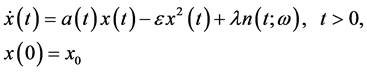 (1)
(1)
where the diffusion coefficient  and initial condition
  are deterministic,
  is a small parameter and
  is the white noise process, whose intensity is given by parameter
 , which has the following important properties:

where E denotes the ensemble average operator,  is the Dirac delta function. And
  is a random outcome for a triple probability space
 , where
  is a sample space, A is a
  -algebra associated with
  and P is a probability measure. The current work also deals with the solution of 2D stochastic quadratic nonlinear equation with
  as non-homogeneity.
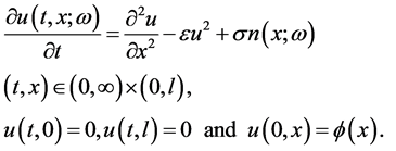 (2)
(2)
where  is the diffusion process,
  is a deterministic scale for the nonlinear term. The non-homogeneity term
  is spatial white noise scaled by
 .
.
The paper is organized as follows. Section 2 summarizes the basic idea of the HAM method. In Section 3, the HAM is applied in order to obtain fourth order approximation of the solution of 1D diffusion model. In Section 4, the HAM is applied up to the third order approximation for the solution of 2D diffusion model. In addition, we compute approximations for the main statistical moments such as the mean and variance. A comparison is done with the results obtained with the (WHEP Cortes [2011], WHEP El-Beltagy [2013]) technique [4,5]. The results are shown in Section 5 along with comments on the results.
2. The Basic Idea of HAM
A presentation of the standard HAM for deterministic problems can be found in [9]. The following subsection is a brief description of HAM. Consider the following differential equation:
 (3)
(3)
where N is a nonlinear operator and  is the unknown function. By means of generalizing the traditional HPM method, Liao [6] constructs the so-called zero-order deformation equation
 (4)
(4)
where  denotes the so-called embedding parameter,
  is an auxiliary parameter and L is an auxiliary linear operator.
The HAM is based on a kind of continuous mapping , where
  is an unknown function,
  is an initial guess for
 , and
, and  denotes a non-zero auxiliary function. It is obvious that when the embedding parameter
  and
and , Equation (3) becomes
 (5)
(5)
respectively. Thus as q increases from 0 to 1, the solution  varies from the initial guess
  to the solution
 . In topology, this kind of variation is called deformation; Equation (3) constructs the homotopy
 .
.
Having the freedom to choose the auxiliary parameter , the auxiliary function
 , the initial approximation
 , and the auxiliary linear operator L, we can assume that all of them are properly chosen so that the solution
  of the zero-order deformation Equation (4) exists for
 .
.
Expanding  in Taylor series with respect to q, one has,
 (6)
(6)
where
 (7)
(7)
Assume that the auxiliary parameter , the auxiliary function
 , the initial approximation
  and the auxiliary linear operator L are so properly chosen that the series (6) converges at
  and
and
 (8)
(8)
which must be one of the solutions of the original nonlinear Equation, as proved by Liao [9]. As  and
and Equation (4) becomes
 (9)
(9)
This is mostly used in the HPM method. According to definition (8), the governing equation and the corresponding initial condition of  can be deduced from the zero-order deformation Equation (4). Define the vector

Differentiating Equation (4) m times with respect to the embedding parameter  and then setting
  and finally dividing them by
 , we have the so-called mth-order deformation equation:
 (10)
(10)
where

and
 (11)
(11)
The solution is computed as:

It should be emphasized that  for
for  is governed by the linear Equation (10) with linear boundary conditions that come from the deterministic problem, which can be solved by any symbolic computation software such as Mathematica, Maple, or Matlab.
3. Application to the 1D Diffusion Model
To demonstrate the above presented method it will be used to find the mean and variance of 1D stochastic diffusion problem as follows.
The auxiliary linear operator will be chosen as

Furthermore, we define the nonlinear operator as

We construct the zero-order deformation equation,

The mth-order deformation equation for  and
and  is
is
 (12)
(12)
Subject to the initial condition

where

Now the solution of the mth-order deformation Equation (12) for  becomes

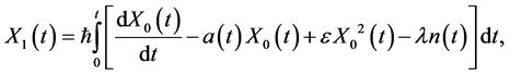
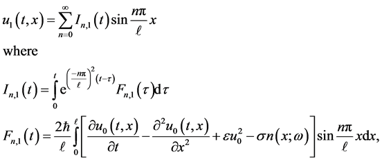
The first order approximation is obtained by setting  in (12) as follows

where

Then

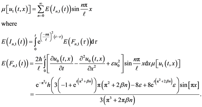
The ensemble average of the first order approximation is

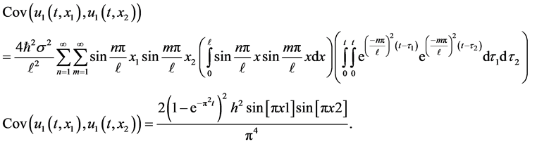
The covariance of the first order solution will be
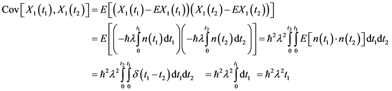
The variance of the first order solution will be

In this manner, we can have more results of  and
and  obtained at
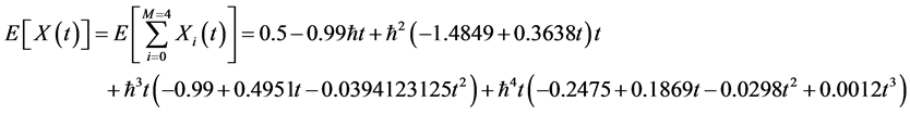
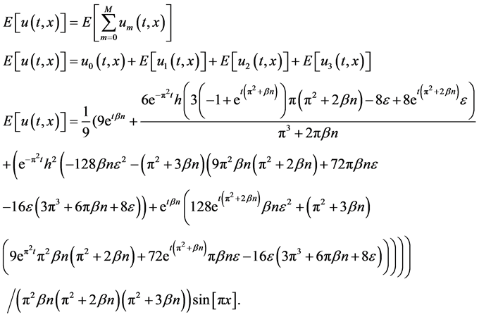
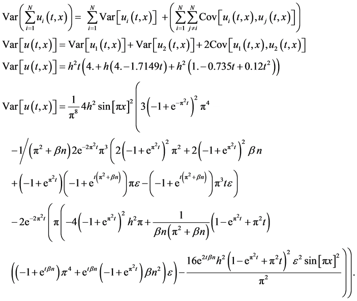
The final expression of the mean of the 4th order solution will be
Since 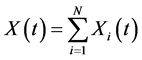
Then the final expression of the variance of the 2nd order solution will be
4. Application to the 2D Diffusion Model
HAM will be used to find mean and variance of stochastic quadratic nonlinear diffusion problem as follows.
The auxiliary linear operator is chosen as

We have many choices in guessing the initial approximation together with its initial conditions which greatly affects the consequent approximation .The choice  is a design problem which can be taken as follows:
 (13)
(13)
One can notice that the selected value function satisfies the initial and boundary conditions and it depends on the parameter  which is totally free. One can also notice that
  selection could control the solution convergence.
Furthermore, we define the nonlinear operator as

We construct the zero-order deformation Equation,

The mth-order deformation Equation for  and
and  is
is

And subject to the boundary conditions

And the initial condition

where

Now the mth-order deformation equation for  becomes

The first order approximation is obtained by substituting  to get
 (14)
(14)
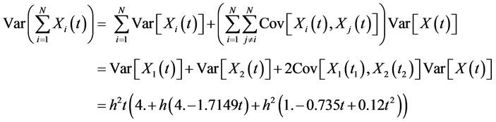
The approximated first order solution of (14) can be obtained using Eigen function expansion as follows,
the ensemble average of the first order approximation is
The covariance of the first order solution can be computed as

The covariance is obtained from the following final expression
The variance of the first order solution will be computed as
 (15)
(15)
To give

In this manner, we can have more results of  and
and  obtained at
The final expression of mean of the 3rd order solution will be
Since 
Then the final expression of the variance of the 2nd order solutionwill be
5. Result Analysis
5.1. 1D Diffusion Model Results
Figures 1 and 2 show the plots of the  -curves for the fourth order variance and mean approximations respectively for different values of time t at
 ,
,  ,
,  and
and  on the time interval [0,]">2]. According to these
  -curves, it is easy to discover that the valid region of
  is a horizontal line segments, thus
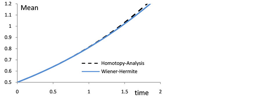
  Figures 3 and 4 show the comparison of the expectation and variance as a function of time using HAM and WHEP which uses the Wiener Hermite expansion and perturbation technique to solve a class of nonlinear partial differential Equations with a perturbed nonlinearity “techniques and good agreement is obtained.
The mean and variance results of the WHEP technique are obtained from [5] as:

The effect of  on the variance is shown in Figure 5. The variance is plotted with time for different values of
 . The peak variance decreases in magnitude with the increase of
 . Also, the time of the peak variance decreases with the increase of
 .
.
5.2. 2D Diffusion Model Results
In the following figures, results of the solution of 2D stochastic quadratic nonlinear diffusion model using HAM technique are shown at ,
, .
.
Figure 6 shows the Plot of  -curve of third order approximation of mean for different values of time t and space variable x at
 ,
, . Figure 7 shows the plot of
  -curve of
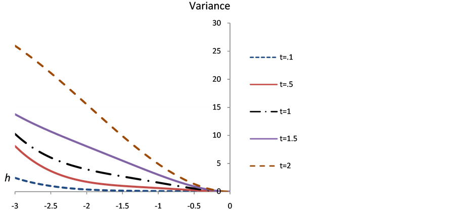
Figure 1. The change of variance of the solution  with parameter
  at different t values.
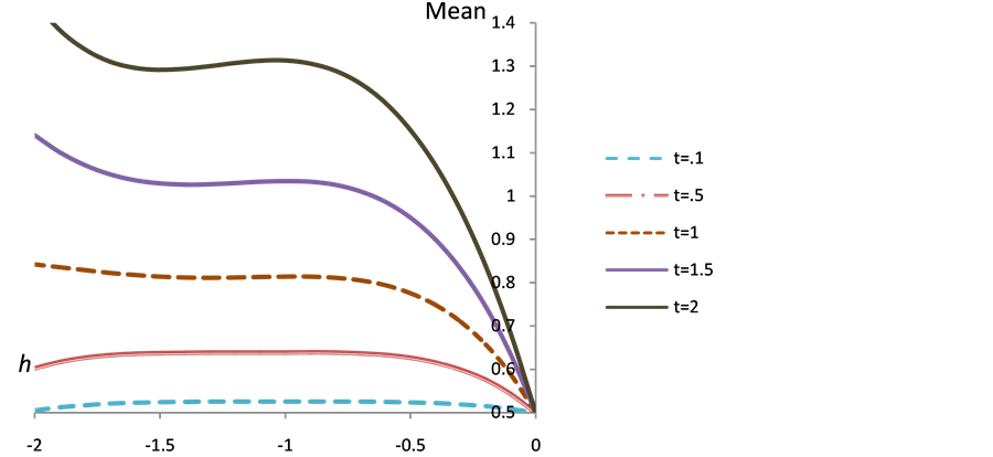
Figure 2. The change of mean of the solution  with parameter
  at different t values.
 for the 1D problem and WHEP
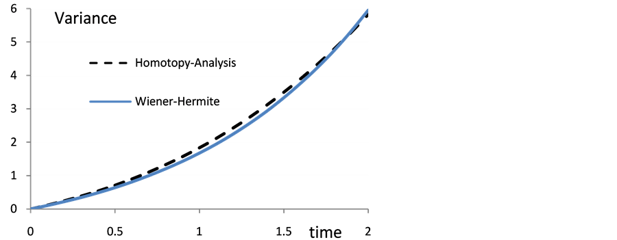
 for the 1D and WHEP
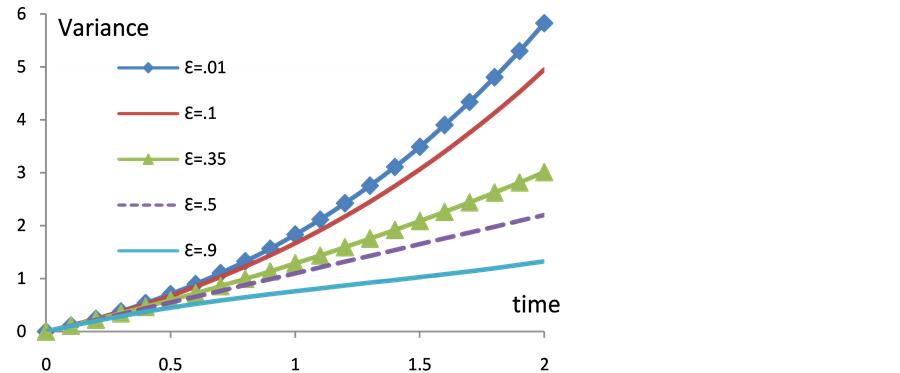
 on Var[x(t)
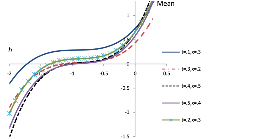
Figure 6. The change of the mean u with parameter  at different t, x values.
third order approximation of mean for different  values. According to these
  -curves, it is easy to discover that the valid region of
  is a horizontal line segments, thus
 . Figures 8 and 9 show the plot of mean and variance with time for different
  values.
Figure 10 shows the comparison between the mean of the first, the second and the third order approximations. Figure 11 shows the comparison between the variance of the first and second order approximations.
6. Conclusion
This paper shows that the HAM technique constitutes a powerful tool for constructing approximate solutions for the stochastic process for random diffusion models with nonlinear perturbations where uncertainty is considered by means of an additive term defined by white noise. The HAM method is employed to give a statistical analytic solution for stochastic 1D and 2D diffusion models. Different from all other analytic methods, the HAM provides us with a simple way to adjust and control the convergence region of the series solution by means of the auxiliary parameter ħ. Thus the auxiliary parameter ħ plays an important role within the frame of the HAM which can be determined by the so called ħ-curves. The solution obtained by means of the HAM is an infinite power series for appropriate initial approximation, which can be, in turn, expressed in a closed form. The accuracy for the method is verified on 1D diffusion model by comparisons with WHEP technique and good agreements are obtained. As shown in Figures 1 and 2, we can see that the valid ħ region in the 1D example is −0.9 < < −1.4 and in 2D example the interval is −0.9 <
  < −1.1, as shown in Figure 6. The results demonstrate reliability and efficiency of the HAM method. Since HAM was used to solve only deterministic problems, we
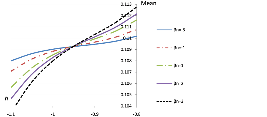
Figure 7. The change of the mean u with parameter  at different
  values,
  , t = x = 0.1.
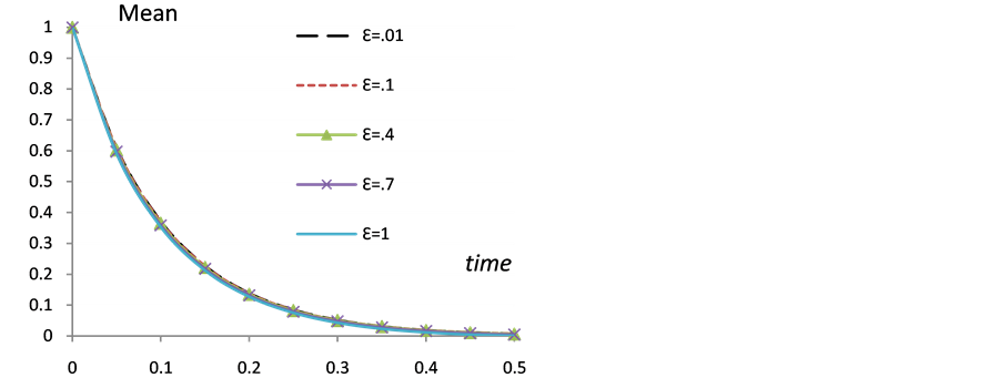
Figure 8. The change of the mean u with time t at different e values, x = 0.1,  ,
, .
.
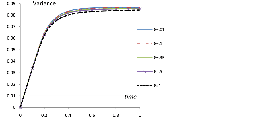
Figure 9. The change of the variance u with time t at different e values, x = 0.1,  ,
, .
.
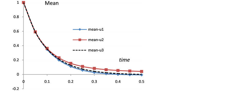
Figure 10. Mean comparison between first u1, second u2 and third order u3 approximations with time t at, x = 0.1,  ,
, .
.
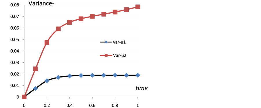
Figure 11. Variance comparison between first and second approximations u1, u2 with time t at, x = 0.1,  ,
, .
.
can say that this is the first time to apply HAM method on stochastic problems and we found that it’s easier than WHEP and more general than HPM since HPM is a special case of HAM obtained at  and its results are accurate.
REFERENCES
- M. A. El-Tawil and A. S. Al-Jihany, “On the Solution of Stochastic Oscillatory Quadratic Nonlinear Equations Using Different Techniques, a Comparison Study,” Topological Methods in Nonlinear Analysis, Vol. 31, No. 2, 2008, pp. 315-330.
- M. A. El-Tawil and N. A. Al-Mulla, “Using Homotopy WHEP Technique for Solving A Stochastic Nonlinear Diffusion Equation,” Mathematical and Computer Modelling, Vol. 51, No. 9, 2010, pp. 1277-1284.
- J. C. Cortes, J. V. Romero, M. D. Rosello and C. Santamaria, “Solving Random Diffusion Models with Nonlinear Perturbations by the Wiener-Hermite Expansion 617 Method,” Computers & Mathematics with Applications, Vol. 61, No. 8, 2011, pp. 1946-1950.
- C. Q. Dai and J. F. Zhang, “Application of He’s Exp-Function Method to the Stochastic mKdV Equation,” International Journal of Nonlinear Sciences and Numerical Simulation, Vol. 10, No. 5, 2009, pp. 675-680.
- M. El-Beltagy and M. El-Tawil, “Toward a Solution of a Class of Non-Linear Stochastic Perturbed PDEs Using Automated WHEP Algorithm,” Applied Mathematical Modeling, Vol. 37, No. 12-13, 2013, pp. 7174-7192. http://dx.doi.org/10.1016/j.apm.2013.01.038
- S. J. Liao, “The Proposed Homotopy Analysis Technique for the Solution of Nonlinear Problems,” Ph.D. Thesis, Shanghai Jiao Tong University, Shanghai, 1992.
- S. J. Liao, “Notes on the Homotopy Analysis Method: Some Definitions and Theories,” Communications in Nonlinear Science Numerical Simulation, Vol. 14, No. 4, 2009, pp. 983-997.
- G. Adomian, “A Review of the Decomposition Method and Some Recent Results for Nonlinear Equations,” Computers and Mathematics with Applications Vol. 21, No. 5, 1991, pp. 101-127.
- J. H. He, “Homotopy Perturbation Method: A New Nonlinear Analytical Technique,” Applied Mathematics and Computation Vol. 135, No. 1, 2003, pp. 73-79.
- T. Hayat and M. Sajid, “Analytic Solution for Axisymmetric Flow and Heat Transfer of a Second Grade Fluid Past a Stretching Sheet,” International Journal of Heat and Mass Transfer Vol. 50, No. 1-2, 2007, pp. 75-84.
- S. Abbasbandy, “Soliton Solutions for the 5th-Order KdV Equation with the Homotopy Analysis Method,” Nonlinear Dynamics, Vol. 51, No. 1-2, 2008, pp. 83-87.
- Y. P. Liu and Z. B. Li, “The Homotopy Analysis Method for Approximating the Solution of the Modified Korteweg-de Vries Equation” Chaos Solitons and Fractals, Vol. 39, No. 1, 2009, pp. 1-8.
- Y. Bouremel, “Explicit Series Solution for the Glauert-Jet Problem by Means of the Homotopy Analysis Method,” Communication in Nonlinear Science Numerical Simulation, Vol. 12, No. 5, 2007, pp. 714-724.
- A. Molabahrami and F. Khani, “The Homotopy Analysis Method to Solve the Burgers-Huxley Equation,” Nonlinear Analysis Real World Applications Vol. 10, No. 2, 2009, pp. 589-600.
- S. Abbasbandy, E. Magyari and E. Shivanian, “The Homotopy Analysis Method for Multiple Solutions of Nonlinear Boundary Value Problems,” Communications in Nonlinear Science and Numerical Simulation Vol. 14, No. 9-10, 2009, pp. 3530-3536.
- H. N. Hassan and M. A. El-Tawil, “Solving Cubic and Coupled Nonlinear Schrödinger Equations Using the Homotopy Analysis Method,” International Journal of Applied Mathematics and Mechanics, Vol. 7, No. 8, 2011, pp. 41-64.
- H. N. Hassan and M. A. El-Tawil, “An Efficient Analytic Approach for Solving Two-Point Nonlinear Boundary Value Problems by Homotopy Analysis Method,” Mathematical Methods in the Applied Sciences, Vol. 34, No. 8, 2011, pp. 977-989.