Received 22 August 2014; revised 16 September 2014; accepted 23 September 2014

ABSTRACT

There has been a growing interest in screening programs designed to detect chronic progressive cancers in the asymptomatic stage, with the expectation that early detection will result in a better prognosis. One key element of early detection programs is a screening test. An accurate screening test is more effective in finding cases with early-stage diseases. Sensitivity, the conditional probability of getting a positive test result when one truly has a disease, represents one measure of accuracy for a screening test. Since the true disease status is unknown, it is not straightforward to estimate the sensitivity directly from observed data. Furthermore, the sensitivity is associated with other parameters related to the disease progression. This feature introduces additional numerical complexity and limitations, especially when the sensitivity depends on age. In this paper, we propose a new approach that, through combinatorial manipulation of probability statements, formulates the age-dependent sensitivity. This formulation has an exact and simple expression and can be estimated based on directly observable probabilities. This approach also helps evaluating other parameters associated with the natural history of disease more accurately. The proposed method was applied to estimate the mammography sensitivity for breast cancer using the data from the Health Insurance Plan trial.

Keywords:

Early Detection of Disease, Screening Test, Sensitivity

1. Introduction

Screening of asymptomatic individuals for chronic diseases is a rapidly growing public health initiative. Early detection programs are aimed at detecting the disease in the stage when a disease is present without symptoms. For example, in breast cancer, there had been eight randomized screening trials demonstrating that mammography screening is beneficial in finding breast cancer at an earlier stage and consequently leads to a decrease in mortality among women of 50 - 65 years of age ([1] -[7] ).

One key element of these programs is a screening test. An important measure for the effectiveness of a screening test is sensitivity (b), the conditional probability of getting a positive screening test result given that one has the disease. Ideally it should be evaluated in the setting of natural history of disease model ([8] -[11] ). Often parameters like the sojourn time distribution in early stage of disease (pre-clinical state), transition probability from no disease state to early-stage disease state are needed to estimate the sensitivity.

These parameters are not directly observable and add to the complexity of the problem formulation and numerical computation of the sensitivity. Furthermore, the sensitivity can be age-dependent. For example in breast cancer the mammogram sensitivity in younger women is lower than that in older women [12] . The formulation for estimating age-dependent sensitivity becomes complex and does not always guarantee a numerical solution.

In this paper, we derive a formula that expresses age-dependent sensitivity in terms of probabilities that are directly observable in screening trials/programs and discuss the characteristics and generalization of this formula. We apply the formula to breast cancer screening trial (Health Insurance Plan) data to estimate the mammography sensitivity [1] .

2. Method: An Exact Expression for Age-Dependent Sensitivity

Consider the following health states in the natural history of disease progression:

· , the disease-free state, when the disease cannot be detected by any current early detection program;

· , the pre-clinical state, when the disease is detectable by an early detection program, but no symptoms are shown; and

· , the clinical state, when symptoms show.

A progressive disease model assumes that the disease progresses in the direction unless it is interrupted by a medical intervention. In the case of chronic progressive diseases, the goal of screening program in detecting the disease in. The age is denoted by a. Let

· be the sensitivity of the screening exam (i.e., the conditional probability that a disease is detected by the screening exam given disease is present) if the exam is taken at age a;

· be the transition rate from to at age a;

· be the sojourn time distribution in if the transition happens at age a; and

· be the probability for case being in the pre-clinical state at age a, i.e. the proportion of people in at age a in absence of screening examinations.

Note that, , and are functions of age a, but to simplify notations, we use a in the subscripts. We also do this in part because our method will give estimates of for discrete values of age a.

We now introduce two important probabilities that all the subsequent derivations are based upon. Suppose there are no screening examinations before age a, and a series of examinations are scheduled (but not necessarily taken) at times at ages, with no examinations at other times. Consider a person of age a at time 0, taking examinations, at times. Let

· be the probability of entering before a, and still be in at age if there has been no screening examinations; and

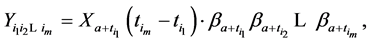
· be the probability for a case undetected by the first exams and being detected in the pre-clinical state at the last examination at time.

The importance of is obvious as it is the probability that can be estimated directly from screening programs by taking proportions. The notion of is more subtle, but it will facilitate derivations which will be shown later, especially when determining and.

Note that it is implied in the definition of T and X that by the time of the last examination, one would either be in or, but not. Thus if we were to use such definitions, we need to limit the cohort to only those who will still be in or by the last examination taken. In fact, the last examination would be at the same time when multiple’s and’s appear in an equation together in all our derivations. Also note that.

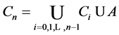
We derive a formula for via a recursion based on the number of examinations. Consider a cohort of age at time 0, with examinations scheduled at times. We have for. n, or the probability of a case undetected at examination at time 0 but at, involves the probability to enter

· before time 0 (or age a), go undetected at time 0, and stay in until getting detected, which is; and

· between time 0 and, and stay in until at least. This can be thought of as the difference between probability to be in at age if there are no exams, or, and the probability to enter before age a and stay in it until age, or. To be detected at, just multiply by, which gives.

Therefore,

Or,

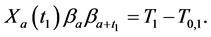(1)

Similarly, for, we need three terms, involving the probability to enter during the following times and stay in until being detected at:

· before age a and go undetected at times 0 and, which is;

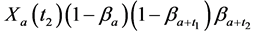· between ages a and and go undetected at age, which is; and

· between ages and, which is.

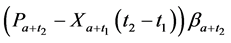Therefore,

From (1), we have 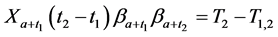and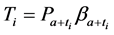, substituting both to the above formulation, we get

which gives

(2)

Observing (1) and (2), we arrive at our main result in this section:

Theorem 2.1.

(3)

Therefore by writing out a few recursions, we are able to eliminate all terms and express the age- dependent as a simple expression of the terms, which are directly observable. A special case for application of Theorem 2.1 is when. This implies a situation where repeated tests are performed on the same individual to measuring the sensitivity. For example, assume up to three repeated tests with the same sensitivity are performed at the same time, at three testing centers with same equipment. We label the testing centers as Center 1, Center 2 and Center 3.

Let be the probability of being detected at Center 1, regardless of what the results from Centers 2 and 3. Let be the probability of being detected by Center 2, but not Center 1, regardless of the result from Center 3. This is equivalent to the probability of being detected by Center 3, but not Center 2, regardless of the result from Center 1. Lastly, let be probability of being detected by Center 3, but not Center 1 or 2. The subtlety here is that is not the probability of being detected by one center out the three, but just 1/3 of it, because we have ordered the centers beforehand. Then we have

Corollary 2.2. When at least three repeated tests with the same sensitivity can be performed at the same time, we have

The result is achieved by simply taking limits and in the derivation for Theorem 2.1.

Theorem 2.1 is far from being intuitive, but corollary is easily verified, when we realize that when and, there is, , and.

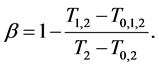
Advantage of Theorem 2.1. One main advantage of Theorem 2.1 is that it enables us to ignore the consideration for transition rate and sojourn time distribution in our set-up, which, even in the simplest cases, creates a complicated relationship. For example, consider the cohort of age 50, all getting their first screening exam. The probability of being detected, if we write it all out as an integral [13] , is

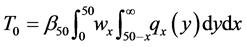
where is the transition probability from to at age and is the sojourn time distribution if the transition happens at age. The interpretation of this expression is straight-forward: to be detected at age 50, the transition needs to happen at some age before 50, therefore the first integral; and needs to last from age to at least age 50, therefore the second integral.

Thus in just this one term, all the’s and’s for less than age 50 are involved, when we do not even know what type of distribution is, which may vary for different’s. This is just the simplest case—when there are multiple exams involved, the expressions for the probability of detection will involve several double integrals. One of the more rigorous approaches by Shen and Zelen ([10] ) uses such expressions to form likelihood function to find estimates for, and. But due to the complexity of such expressions, even when age-dependency is ignored, and is assumed to be exponential (so there are only three parameters to determine:, and the parameter for the exponential), there is no guarantee that a global maximum exists, or can be determined [11] .

However Theorem 2.1 allows us to bypass and and find an expression for in as an exact expression of’s. This, of course, does not mean that the effects of on detection can be isolated from that of and, but that the information of and are already incorporated in the’s. We also want to point out that the’s involved in Theorem 2.1 are naturally observable probabilities in the case of breast cancer screening (which is the main area of study for the authors): it is recommended that women to be screened either once every year, which gives terms, , or once every other year, which gives term.

Another important advantage of Theorem 2.1 is that once (age-dependent) is determined, we will be able to determine age-dependent w and q with various approaches in a more exact manner. This we will explore in another paper.

One limitation of the Theorem 2.1 is that it does not provide a way to apply the “interval cases”, or the cases that enter clinical stages between two scheduled screening exams. These cases, however, can be used later on to determine w and once is determined.

3. Symmetry between X and T

An interesting mathematical result involves certain symmetry between X and T. We use the same setup as in the last section: suppose there are no examinations before age a, and a series of exams are scheduled (but not necessarily taken) at times 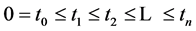at ages, with no examinations at other times. Consider a person of age a at time, taking m examinations at times. Recall that we let be the probability for the person to be undetected by all of the first exams and only detected to be in the pre-clinical stage at the last exam at time.

Under the same set up, we introduce the new notation:

(4)

where is the probability for someone to enter before age and still being in at age, if there has not been any medical intervention. Thus is the probability for such a patient being detected at examinations taken at times. This is a hypothetical probability that will facilitate our derivation.

We also recall how we have defined: let be the probability for the person to be undetected by all of the first exams and only detected to be in the pre-clinical stage at the last examination at time. So the onset of can happen anytime before, as compared to in the definition of (and therefore), where the onset of occurs before age.

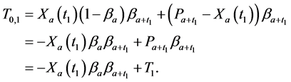
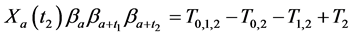
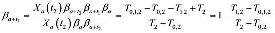
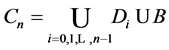
Recall we derived the following expressions in the last section (notice that):

or, after some reorganizing of the terms, and recognizing that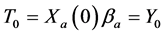, we have

Therefore it is clear that there is a symmetric relationship between the T terms and the corresponding Y terms, in the case of 1, 2 and 3 examinations. The pattern of these expressions becomes more obvious in case of 4 examinations: (which will be proved along with the general case) to make it more obvious:

In the expression of in terms of the Y terms (and vice versa), the subscripts of Y terms go though all the eight subsets of union 3, and the sign in front of the Y terms alternate according to the size of the subset. These facts turn out to be universal. We have:

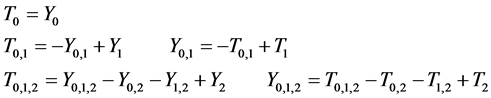
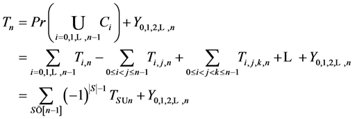
Theorem 3.1. For any, there is

and

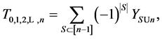
where S goes over all subsets of, including the empty set, and is the size of S.

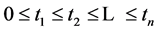
Proof. Because we will be applying the inclusion-exclusion principle later, to make the corresponding arguments, we revise the definition of the’s slightly. Assume a series of examinations are scheduled at times at ages, , , with no examinations at other times. However, assume that all the examinations are taken (again it is implied that one is still in either or by the time, i.e., we limit to the cohort of such), and not all results are taken into consideration. Therefore even if has been detected at time , all the subsequent examinations will still be taken. Let be the probability for the person be the probability for an individual undetected by the examinations at times, and detected in at exam, regardless of what happens at other examinations. Although the definition for’s has changed, the numerical expression of’s are the same as before.

Let

· be the event of being detected at but undetected at;

· be the event of being detected at;

· be the event of being detected at all exams at.

Therefore we have

and 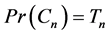(which is also equal to), while the size of the right-hand-side would be

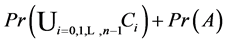, since A and each C_i are mutually exclusive events. We also have.

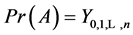By inclusion-exclusion principle [14] ,

But 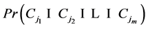is simply, therefore we have

Or,.

The second expression can be proved in a similar manner. With the same set up as the above, let

· be the event of being detected by two examinations at and at;

· be the event of being undetected by every examination taken at, but detected at.

Recall that is the subset of all those detected at, then

and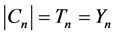. While this time the size of the right-hand-size is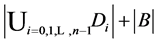, since B and each are mutually exclusive events. We also have.

Again by inclusion-exclusion principle,

However 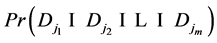is simply, therefore we have

Or,.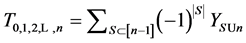

Corollary 3.2. There are infinitely many expressions of age-specificity in terms of.

Proof. This is because each can be expressed as

where is any subset of that contains, and means without. For example,

we saw in the last section that, and it is also equal to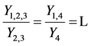, etc.

Each can be expressed in terms of’s.

Given expressions like Theorem 3.1, the proof for Theorem 2.1 is not as straightforward. However the purpose of that proof was to relate some of the traditional considerations and reasoning’s to our new notions. This will be useful when evaluating important parameters such as age-dependent disease transition probabilities and sojourn time distribution.

4. An Example

We illustrate the proposed method using the data from the Health Insurance Plan Project, or HIP data [1] . HIP is a randomized screening trial of mammography screening vs. no screening for the women who did not have previous mammography. Even though HIP is a large-scale screening trial, because breast cancer incidence rate is relatively low, we do not have sufficient number of screen-detected and interval cases to readily estimate age-specific. Thus for an illustration of the Theorem 2.1, we group all the women together as one age group, and assume that all patients had the same age at the initial examination. Because the cohort is required to have annual check-ups, we set and in the Theorem 2.1, and get

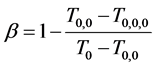
To calculate, saying, we simply use the ratio between the number of cases detected at the first annual examination after the initial examination and all the cases who had taken both examinations. Using the HIP data, we get

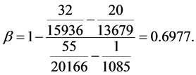
Note that this estimate is essentially identical to Shen and Zelen’s published estimate of 0.7 ([10] [11] ) based on the maximum likelihood method, but is computationally trivial.

Acknowledgements

This work was supported by grants 1RC CA 146496-01 and 1R01 CA16430 from the National Cancer Institute/National Institute of Health.

References

NOTES

^*Corresponding author.

References

- Shapiro, S., Venet, W., Strax, P., et al. (1988) Periodic Screening for Breast Cancer: The Health Insurance Plan Project and Its Sequelae, 1963-1986. The Johns Hopkins University Press, Baltimore.
- Tabar, L., Gunnar, F., Duffy, S.W., et al. (1992) Update of the Swedish Two-County Program of Mammographic Screening for Breast Cancer. Radiologic Clinics of North America, 30, 187-210.
- Andersson, I., Aspegren, K., Janzon, L., et al. (1988) Mammographic Screening and Mortality from Breast Cancer: The Malmo, Mammographic Screening Trial. British Medical Journal, 297, 943-948. http://dx.doi.org/10.1136/bmj.297.6654.943
- Frisell, J., Glas, U., Hellstrom, L., et al. (1986) Randomized Mammographic Screening for Breast Cancer in Stockholm. Breast Cancer Research and Treatment, 8, 45-54. http://dx.doi.org/10.1007/BF01805924
- Bjurstam, N., Bjorneld, L., Duffy, S.W., et al. (1997) The Gothenburg Breast Screening Trial: First Results on Mortality, Incidence, and Mode of Detection for Women Ages 39 - 49 Years at Randomization. Cancer, 80, 2091-2099. http://dx.doi.org/10.1002/(SICI)1097-0142(19971201)80:11<2091::AID-CNCR8>3.0.CO;2-#
- Roberts, M.M., Alexander, F.E., Anderson, T.J., et al. (1990) Edinburgh Trial of Screening for Breast Cancer: Mortality at Seven Years. Lancet, 335, 241-246. http://dx.doi.org/10.1016/0140-6736(90)90066-E
- Miller, A.B., Baines, C.J., To, T., et al. (1992) Canadian National Breast Screening Study 1: Breast Cancer Detection and Death Rates among Women Aged 40 to 49 Years. Canadian Medical Association Journal, 147, 1459-1476.
- Duffy, S.W., Chen, H., Tabar, L. and Day, N. (1995) Estimation of Mean Sojourn Time in Breast Cancer Screening Using a Markov Chain Model of Both Entry to and Exit from the Preclinical Detectable Phase. Statistics in Medicine, 14, 1531-1553. http://dx.doi.org/10.1002/sim.4780141404
- Paci, E. and Duffy, S.W. (1991) Modeling the Analysis of Breast Cancer Screening Programmes: Sensitivity, Lead Time and Predictive Value in the Florence District Programmes (1975-1986). International Journal of Cancer, 20, 852-858.
- Shen, Y. and Zelen, M. (1999) Parametric Estimation Procedures for Screening Programmes: Stable and Non-Stable Disease Models for Multimodality Case Finding. Biometrika, 86, 503-515. http://dx.doi.org/10.1093/biomet/86.3.503
- Shen, Y. and Zelen, M. (2001) Screening Sensitivity and Sojourn Time from Breast Cancer Early Detection Trials: Mammograms and Physical Examinations. Journal of Clinical Oncology, 19, 3496-3499.
- Tabar, L., Fagerberg, G., Chen, H., et al. (1995) Efficacy of Breast Cancer Screening by Age. Cancer, 75, 2507-2517. http://dx.doi.org/10.1002/1097-0142(19950515)75:10<2507::AID-CNCR2820751017>3.0.CO;2-H
- Zelen, M. (1993) Optimal Scheduling of Examinations for the Early Detection of Disease. Biometrika, 80, 279-293. http://dx.doi.org/10.1093/biomet/80.2.279
- Stanley, R.P. (1999) Enumerative Combinatorics, Vol. 1. Cambridge University Press, Cambridge. http://dx.doi.org/10.1017/CBO9780511609589