Applied Mathematics
Vol.4 No.5(2013), Article ID:31570,10 pages DOI:10.4236/am.2013.45115
Finite Difference Preconditioners for Legendre Based Spectral Element Methods on Elliptic Boundary Value Problems*
1Department of Mathematics, Kyungpook National University, Daegu, South Korea
2Computation and Modeling, Shell Technology Center Houston (STCH), Houston, USA
Email: seonykim@knu.ac.kr, Amik.St-Cyr@shell.com, #skim@knu.ac.kr
Copyright © 2013 Seonhee Kim et al. This is an open access article distributed under the Creative Commons Attribution License, which permits unrestricted use, distribution, and reproduction in any medium, provided the original work is properly cited.
Received November 13, 2012; revised April 1, 2013; accepted April 8, 2013
Keywords: Finite Difference Preconditioner; Iterative Method; Spectral Element Method; Elliptic Operator
ABSTRACT
Finite difference type preconditioners for spectral element discretizations based on Legendre-Gauss-Lobatto points are analyzed. The latter is employed for the approximation of uniformly elliptic partial differential problems. In this work, it is shown that the condition number of the resulting preconditioned system is bounded independently of both of the polynomial degrees used in the spectral element method and the element sizes. Several numerical tests verify the h-p independence of the proposed preconditioning.
1. Introduction
Linear systems engendered by spectral element discretizations of a simple second-order elliptic boundary value problem have large condition numbers depending on the number of elements E and the polynomial degree N employed. Convergence of iterative solvers thus deteriorates as E and N increases. Regardless of these restrictions, the spectral element method is very popular, accurate and used in many engineering problems. However, it is widely known that an efficient preconditioner is necessary in order to improve the convergence of Krylov subspace methods traditionally used to solve the resulting linear system (see [1-7]). Since the work of [8], it is numerically known that finite difference preconditioning of the spectral element matrix leads to satisfactory results in terms of convergence rates. Multigrid methods are optimal in terms of convergence rate and have linear cost for finite difference problems. The Algebraic multigrid (=: AMG) method can be easily applied to finite difference discretizations of elliptic operators. If it is instead applied directly to high-order discretizations, such as spectral elements, some outstanding issues still need to be addressed. The idea of employing a low-order discretization combined with multigrid as the preconditioner of a high-order problem was investigated in [9] where P1 finite elements were employed instead of finite differences. Other efforts concerning the computational cost of P1 finite element based two levels additive Schwarz preconditioners can be found in [10,11]. In both approaches an intermediate problem for the Laplace equation was constructed using the high-order Legendre-Gauss-Lobatto (=: LGL) nodes. Furthermore, analytic work was performed in [12] for a second-order uniformly elliptic boundary value problem using LGL nodes and also the analytic research based on Chebyshev-Gauss-Lobatto (=: CGL) nodes was done in [13], in which the various node configurations (LGL and CGL nodes) were employed for the construction of the P1 finite element preconditioner. In the 1- and 2-dimensional case, the approach was proven optimal and scalable, respectively.
Thus an efficient and optimal algorithm, with linear cost, for solving problems based on spectral element discretizations, which guarantees the convergence of the overall preconditioning strategy, is readily available. The P1 finite element matrix lowers the complexity of the system to invert since the matrices, representing the Laplacian, are tri, penta or hepta diagonal and are easily solvable using the multigrid method.
Recently Canuto et al. [14,15] have discussed preconditioning with low order finite-elements methods. They show the equivalence between spectral elements and low order finite-elements. The proof is shown for finite-elements and so called numerical integration (NI). In our approach, following motivations found in [4], we propose another preconditioning approach using a simple finite difference scheme based on the LGL nodes in a pointwise approximation perspective. The latter is represented as tensor product matrices, and finite element related properties are employed to prove its optimality. Additionally, it is shown that the proposed preconditioners herein are optimal from the theoretical analysis standpoint and that optimality is confirmed with numerical experiments.
The paper is organized as follows. First, the problem is described in Section 2 and basic definitions are recalled in the same Section 2 also. In the same section, the finite difference preconditioner is introduced. In Section 3, a uniform bound for , the ratio of LGL weights to the distance between the adjacent LGL nodes, is derived which will be used for the 2D case. The optimality results are presented in Sections 4 and 5 with the numerical experiments which support the developed theories. Finally, conclusions are drawn.
2. Description of the Problem
Consider the classical boundary value problem of a second-order elliptic operator
 (2.1)
(2.1)
where  and
and  are satisfying
 (2.2)
(2.2)
The resulting matrix for the operator A, with variable coefficients, discretized using spectral element methods based on LGL nodes is represented as  and
and  in oneand two-dimensional case, respectively. Twodimensional matrix
  is the result of tensor products using the matrices obtained in the one-dimensional case. We shall consider the preconditioner
  and
and  for the 1D and 2D case, respectively. Then the problem is to demonstrate the validity of the preconditioners
  for
for  and
and  for
for , respectively. Moreover, the goal is to show that the preconditioners are optimal in the sense that the condition numbers of the preconditioned systems
  and
and  for each case are independent of mesh sizes
  of elements and degrees
  of the piecewise polynomials employed in spectral element discretization.
For the above goal, we will introduce some notations and definitions from now on. Let ![]() and
and ![]() be the reference LGL points in
be the reference LGL points in  and quadrature weights associated with the
  -degree Legendre polynomial. With dimensionless notations t, let us denote
  as the knots in the interval
  such that
  For convenience, we denote
  as the degree of Legendre polynomial on each subinterval
 .
.  will be the sum of the degrees of each element up to k:
 . In particular, the notation
  is used when k = E and
 . The translated LGL points and corresponding weights from
 ![]() and
and ![]() are
are
 with
with
 (2.3)
(2.3)
and, respectively, :
:
 (2.4)
(2.4)
and 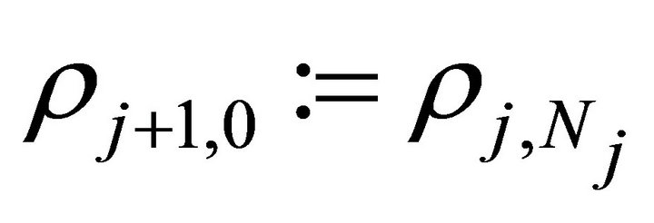 for
for .
.
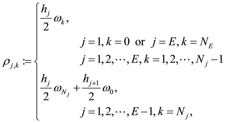
For simplicity, all LGL points  are arranged as
 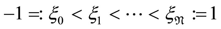 and the corresponding LGL weights are ordered as
  with
with
 . Notice that from (2.3)
  for
for  follows.
Let  be the space of all polynomials
  defined on
  whose degrees are less than or equal to k and let
  be the subspace of
 , which consists of piecewise polynomials
  with support
  whose degrees are less than or equal to
 . Let
. Let  be the space of all piecewise Lagrange linear functions
  with respect to
 ![]() on
on . Define
  as the space of all Lagrange piecewise linear functions
  with respect to
![]() . Let
. Let  be the standard Sobolev space with zero boundary conditions. Let
  and
and
 be the finite dimensional subspaces of
 with the basis functions
  and
and ![]()
respectively, where . To communicate between the space of piecewise linear functions and the space of piecewise polynomial, we use the interpolation operator
  such that
  for
for .
.
For the two-dimensional case, the LGL points are reordered by horizontal lines or, more precisely, all the points are listed as , where
 for
for ,
, . For the two-dimensional high-order and piecewise linear space, let

and

whose basis functions are given by tensor products of one-dimensional piecewise Lagrange polynomials and linear functions, respectively. Let .
.
Note that , where
 ,
,  or
or![]() .
.
To provide the preconditioner, using the global LGL points , we define the operator
  on
on 
 (2.5)
(2.5)
where ,
, .
.
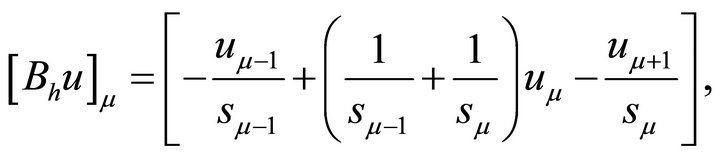
With this operator and components ,
,  , we define the one-dimensional finite difference operator
  as following:
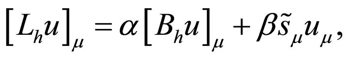
where .
.
The two-dimensional finite difference operator  is therefore defined as
 (2.6)
(2.6)
where  is the 2D version of (2.5) for
  or y, precisely,
 (2.7)
(2.7)
and ,
,  for
for  or y and
 .
.
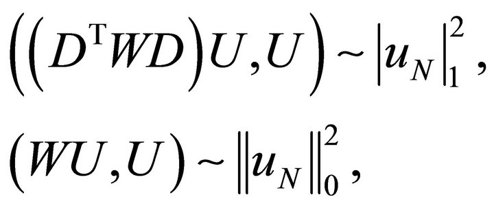
Finally, the notation  for any two real quantities a and b is a shorthand notation corresponding to the existence of two positive constants c and C, which do not depend on the mesh sizes and the degrees of polynomials such that
  The notation (U, V) stands for
  for any two vectors
  and
and  where the superscript T denotes the transpose of a vector or matrix. The standard Sobolev space H1 and L2 will be used. And we will use
 ,
,  and
and  as the standard Sobolev H1-norm, H1-seminorm and the usual L2-norm, respectively.
3. Basic Estimates
We begin by recalling the relations between the distances of LGL nodes and the LGL weights in the reference element  found in [6].
Lemma 3.1. With LGL nodes  and LGL weights
 , let
, let
 (3.1)
(3.1)
 (3.2)
(3.2)
Then the  are uniformly bounded for all
  . In particular,
 (3.3)
(3.3)
where  are constants independent of the polynomial degree N.
Proof. See Lemma 3.1 in [6]. □
Since the goal is to develop preconditioners on spectral elements considering different polynomial degrees on each elements of which sizes are not identical, we need an advanced version or ![]() -version of Lemma 3.1. Hence the modifications of (3.1)-(3.2) for
-version of Lemma 3.1. Hence the modifications of (3.1)-(3.2) for
 are required, where
 .
.
First, let ,
,  and
and 
 be defined as
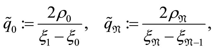 (3.4)
(3.4)
and
 (3.5)
(3.5)
Lemma 3.2. The  given in (3.4)-(3.5) are bounded for all
  independently of both degrees
  of polynomials and the mesh sizes
  of each element.
Proof. Since the LGL nodes in each subinterval are defined by an affine map transformation from the ones in reference interval , they depend on the mesh sizes of each element thus they are distinguished as follows

(3.6)
Since the first and second cases of (3.6) are
and

it is clear that ,
,  are uniformly bounded by Lemma 3.1.
For the case ,
,  , it can be easily shown that
Lastly for ,
,  , note that
Using (3.3), it comes
and
 where
where  are the absolute positive constants that appear in Lemma 3.1. Therefore,

which completes the proof. □
Define the two matrices W and H, which are made up of, respectively, the quadrature weights and the distances between the LGL points:
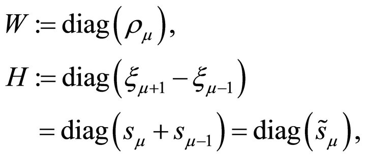 (3.7)
(3.7)
where  and
and .
.
Notice that the quantities  and
and  are positive for all
 . By Lemma 3.2,
  defined in (3.5) are uniformly bounded. Thus we have the following corollary:
Corollary 3.3. For , it follows that
The next result is a clear consequence but we write down for convenience.
Lemma 3.4. For any diagonal matrix S with nonnegative entries whose size is the same as W (see definition in (3.7)),

where the equivalence depends on the minimum and maximum entries of S.
The matrix W will be replaced by  for twodimensional problems.
Proposition 3.5. Let  be symmetric and positive definite matrices such that
 (3.8)
(3.8)
for any nonzero vector . Then for any symmetric and positive definite matrix
 , we have
 (3.9)
(3.9)
Proof. Since all the matrices are symmetric and positive definite, it is enough to discuss (3.9) in terms of eigenvalues.
Consider the eigenvalue problem
It has a complete set of eigenpairs ,
,  . Let
. Let
 (3.10)
where 1 is a vector consisting of element 1 with length .
.
Since
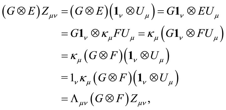
the vectors and eigenvalues in (3.10) are complete sets of eigenvectors and eigenvalues of the eigenvalue problem
From (3.8), since  are positive, bounded and independent of
 ,
,  , so are
 . Therefore it follows

By the same reasoning, it follows
 . □
. □
Finally, the known results stated in Theorem 3.3 and 3.5 from [12] are recalled here for completeness.
Theorem 3.6. It follows that for all ,
,
![]()
4. One-Dimensional Case
Before going ahead, suppose that  and
and  satisfy
  and
and  , where
 ,
,  ,
,  and
and  are constants. Now consider the following elliptic boundary value problem with zero boundary condition:
 (4.1)
(4.1)
Expanding  and
and  in (4.1) on the space
  as
as ![]() and
and![]() , the matrix representation of the operator A in (4.1) by the spectral element discretization based on LGL points is now given by
, the matrix representation of the operator A in (4.1) by the spectral element discretization based on LGL points is now given by
 (4.2)
(4.2)
where ,
,  , D is the differentiation matrix defined as
  and W is the matrix defined in (3.7).
Since P and Q are the diagonal matrices with nonnegative elements, by Lemma 3.4 we have for any vector U,
and
More precisely, it follows that
 (4.3)
(4.3)
 (4.4)
(4.4)
Besides, we can see that for
![]() ,
,
 (4.5)
(4.5)
where .
.
Let  be the matrix representation of
 , which is defined in (2.5). For
![]() , the easy calculation leads to
, the easy calculation leads to
 (4.6)
(4.6)
where .
.
Note that the constants such as ,
,  appeared in this and next sections are generic positive constants, independent of the number of elements
  and the degree
  of polynomials applied to spectral discretization.
Now to provide a finite difference type preconditioner, consider the bilinear form  with a positive constant
![]() , defined on the space
, defined on the space 

where . This induces the matrix
 :
:


Thus it comes immediately
 (4.7)
(4.7)
Lemma 4.1. For any vector , it follows that
Proof. Note that  can be expressed as
![]() , so that its piecewise polynomial interpolation becomes
, so that its piecewise polynomial interpolation becomes![]() .
.
Since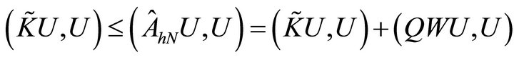 , it follows from (4.3)-(4.5), that
The last inequality is due to Poincare’s inequality. Therefore, (4.7), (4.6) and Theorem 3.6 complete the proof. □
Remark 1. From the above lemma, one may notice that the upper bound for the condition numbers of the matrix  does not depend on the mesh size hj of an element and the degree Ni of a polynomial. Further, it does not depend on
![]() . Hence, even if (4.1) has coefficient functions
. Hence, even if (4.1) has coefficient functions  and
and , it is enough to take the preconditioner
  with
with  in (4.7).
Next, we consider another bilinear form  on the space
  with a constant
where  and
and . The matrix representation
  corresponding to
  is
is


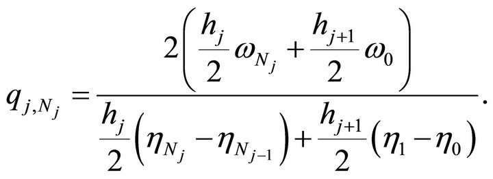
where
 (4.8)
(4.8)
Now the goal is to analyze the validity of the matrix operator  for the preconditioner to
 .
.
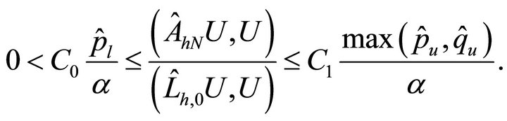
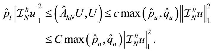
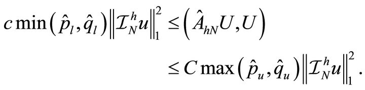
Theorem 4.2. For any vector , it follows that
where the equivalence depends only on ,
,  ,
,  ,
,  ,
, ![]() and
and .
.
Proof. For  such that
![]() , its piecewise polynomial interpolation is
, its piecewise polynomial interpolation is
![]() . Using (4.3)-(4.5), we get
. Using (4.3)-(4.5), we get
On the other hand, applying Corollary 3.3, (4.5) and Theorem 3.6 we have
![]() (4.9)
(4.9)
so that

Hence, using Theorem 3.6 again, we have
To guarantee the positivity of the lower bound, if , we will take
 . Applying Poincare’s inequality with (4.9) and (4.6), we have
 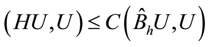 for some positive constant C. Therefore, using (4.3)-(4.5) and Theorem 3.6, we get
so that
which leads to the conclusion.
The latter, combined with the min-max theorem, yields the next result.
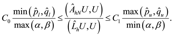
Corollary 4.3. The eigenvalues  of
of  are all positive real and bounded above and below. The bounds are independent of the mesh sizes hj and the degrees of the polynomials Nk. That is, there are absolute constants
  and
and  such that
Remark 2. Theorem 4.2 reveals that the condition numbers of  are bounded above by
 or
or . Hence one may notice that the condition numbers do not depend on the degrees of polynomials
  and the mesh sizes
 .
.
According to Remark 2, we may summarize the behavior of the condition numbers of  in the following corollary.
Corollary 4.4. The upper bound of the the condition numbers of  behaves like
 ,
,  ,
,  or
or .
.
We will investigate the efficiency of the preconditioners  and
and  for several problems with constant and variable coefficients. Moreover, for a variable coefficients problem, we will compare the developed preconditioners with the
  finite element preconditioner (see [12]) in terms of iteration numbers using the preconditioned conjugate gradient method (=: PCG).
Example 1. Consider the operator with constant coefficients:
 (4.10)
with homogeneous Dirichlet boundary conditions, where  and
and  are constants. Note that the spectral element discretized matrix corresponding to (4.2) becomes
 . Since the condition numbers are dependent on the ratios
 ![]() and
and ![]() by the definition, we take
by the definition, we take  and focus mainly on the role of
 , where
 .
.
First, it is computed with . Figure 1 is shown to be ineffective for large values
![]() , but we can see that
, but we can see that  is effective for
 ![]() -value equal or less than 1 (see Table 1).
-value equal or less than 1 (see Table 1).
Second, to show that the preconditioning work is not independent of the polynomial degrees N and the numbers of element E, applied in spectral element method, it is tested for the cases with  and
and  . For the values
 , the condition numbers of
 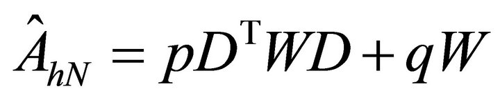 go up to approximately
  when
when , but ones of the matrices preconditioned by
  are bounded above by approximately 4.5, independently of N, E (see Figure 2).
Third, We investigated the condition numbers of the matrices by preconditioned by  with several
  -values for each
 ![]() -value (see Figure 3). When
-value (see Figure 3). When  is taken to be equal to
 ![]() -value or
-value or , it gives good preconditioning results (see Figure 4).
Example 2. Now we consider the operator with the variable coefficients:
 (4.11)
with homogeneous Dirichlet boundary conditions, where  and
and , where
  and
and  are constants. In this case, the spectral element discretization yield the matrix
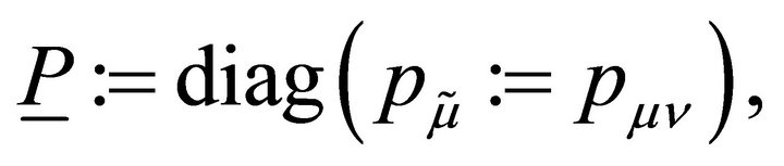
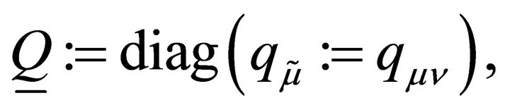
 , where P and
  are the matrices of
  and
and ![]() represented by spectral
represented by spectral

Figure 1. Condition numbers of , where
 .
.

Table 1. Condition numbers of , where
 .
.
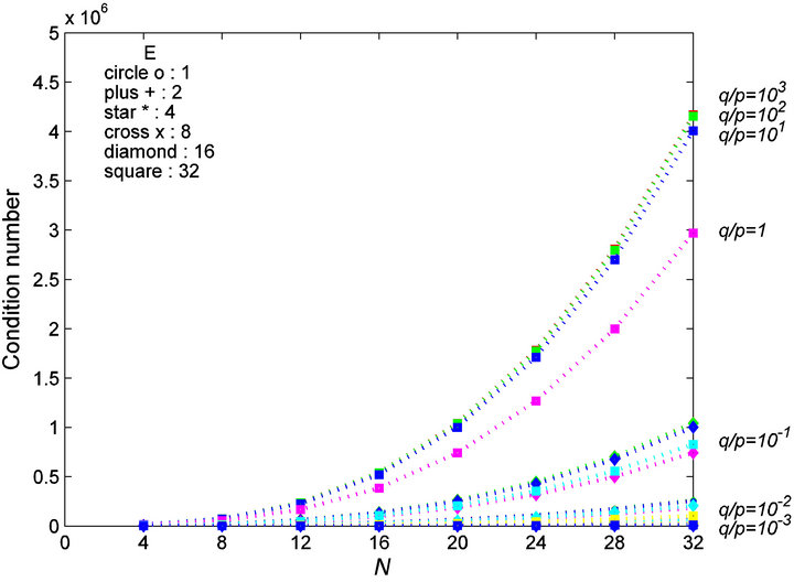
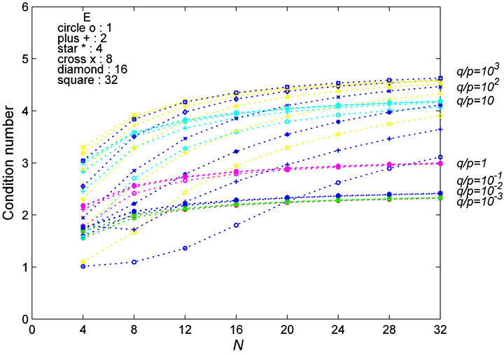
Figure 2. Condition numbers of  and
and , where
 .
.
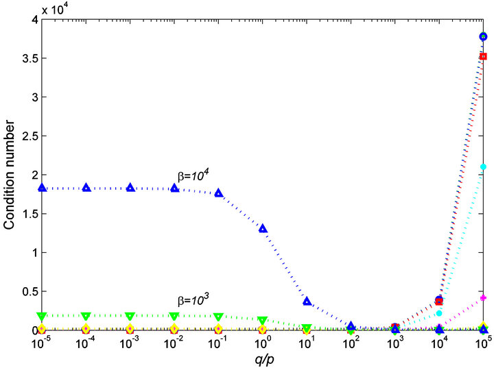
Figure 3. Behaviors of![]() , where
, where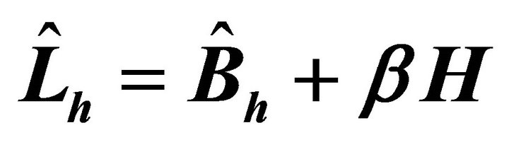 .
.
element discretization, respectively. Figure 5 shows that  or
or 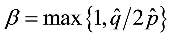 give the good preconditioning results.
Example 3. For the variable coefficients problem of Example 2 with  and
and :
:
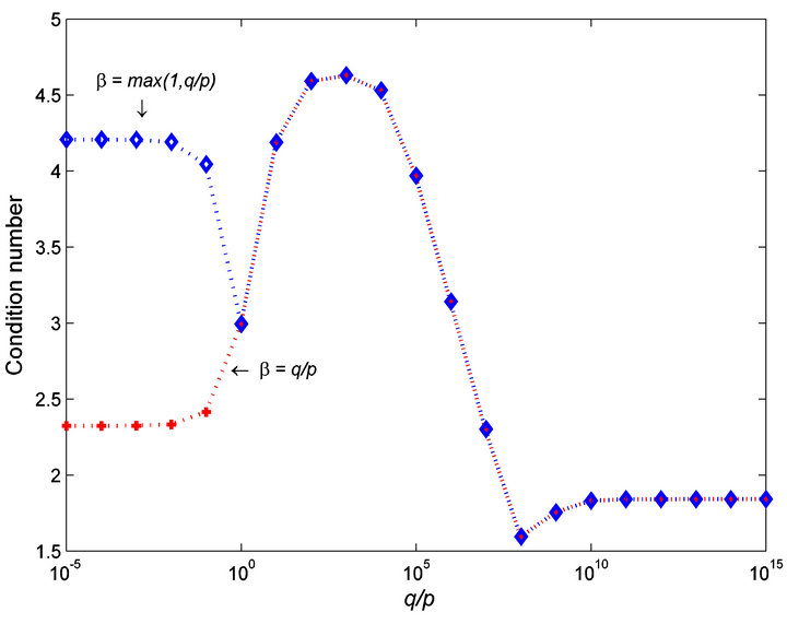
Figure 4. Condition numbers of , where
  βH.
βH.
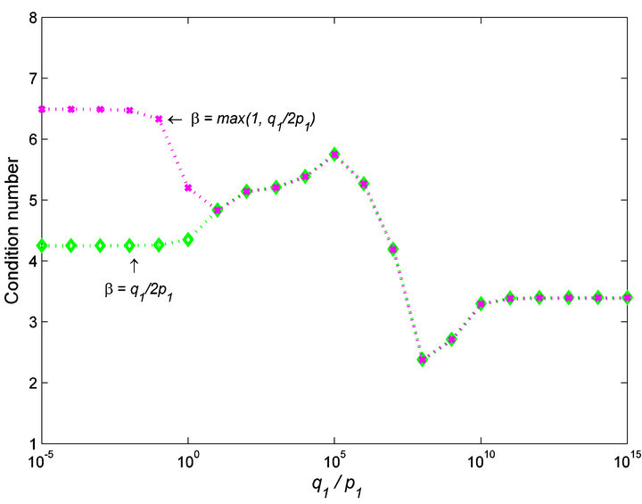
Figure 5. Condition numbers of , where
  βH.
βH.
 (4.12)
we compute the iteration number using PCG preconditioned by . Also we compare the developed preconditioners
  with the
  finite element preconditioner
  (see [10,12] for example) in terms of iteration numbers using PCG.
The computational results are shown in Table 2 with various numbers of elements E and polynomial degrees N. While the number of iterations increases as N or E becomes large in case of CG iterations, the PCG preconditioned by  gives relatively small. In particular, it can be predicted that the preconditioning effects become stronger as N or E are made larger. Furthermore we note that the results are comparable to the ones for finite element preconditioner.
5. Two-Dimensional Case
In this section the tensor notation is employed. It has the form  and the superscripts denote the spatial dimension on which it acts. Their order will always be the same and thus we omit them. For the tensor product representation, we refer to [16].
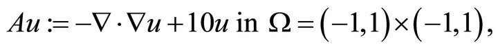
Consider the elliptic operator corresponding to 2D case with zero boundary conditions:
 (5.1)
(5.1)
where  and
and  are satisfying
  ,
, .
.
As in the 1D case, by expanding the variable coefficients  and
and  in terms of the basis
 of
of , two coefficients matrices are obtained:
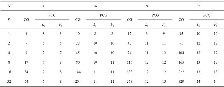
Table 2. Iteration numbers in 1D.

Then the matrix from the spectral element discretization, using one-dimensional matrices D and W, becomes
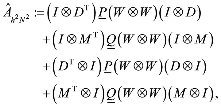 (5.2)
(5.2)
where  is the 1D mass matrix, which becomes the identity for the Lagrange basis
 .
.
From the similar argument in 1D case such as (4.3)- (4.4), we have

for any nonzero vector .
.
In order to describe the preconditioner for the  case, with the operator
  defined in (2.6), we consider a bilinear form
  on
on 
which becomes
where
 (5.3)
(5.3)
and  is the matrix induced from (2.7) for each
  or
or![]() .
.
Notice that in the proof of Lemma 4.1 it is shown that  is for any nonzero vector
 . Using this fact and Proposition 3.5, we have the following:
Theorem 5.1. For any vector , we have

where the equivalence are dependent only on ,
,  ,
,  ,
,  ,
, ![]() and
and .
.
Hence, the eigenvalues of  are all positive and bounded. The bounds are independent of the mesh sizes
  and the degrees
 , where
  or
or![]() .
.
Remark 3. This result reveals, as in  case, that the upper bound for the condition numbers of the matrix
  is dependent only on the variable coefficients
  and
and , precisely the condition numbers are bounded above by
  or
or  .
.
In the following example, the various eigenvalues and condition numbers of the preconditioned matrix are reported. They are compared with their  finite element sibling. Also included is a comparison of the iteration counts, for a PCG solver, for the proposed preconditioners.
Example 1. Consider the homogeneous Dirichlet boundary value problem

where  and
and
 .
.
As in 1D case, we consider  or
or  to have a good preconditioning work, which are shown in Figure 6.
Example 2. For the homogeneous Dirichlet boundary value problem
we now compare the developed preconditioners  with the
  finite element preconditioner
  in terms of iteration numbers using the PCG.
As in the 1D case, we compare the number of PCG iterations for the preconditioners  and
and  which is provided in [12]. In Table 3, we can see that the suggested finite difference preconditioner
  is more
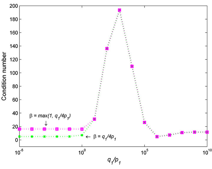
Figure 6. Condition numbers of .
.

Table 3. Iteration numbers in 2D.
efficient as compared to the  finite element preconditioner
 .
.
6. Conclusion
We have proposed finite differences preconditioners  and
and  for spectral element discretizations, and constructed on LGL nodes for uniformly elliptic problem in n-dimension,
  , respectively. The two preconditioners optimality for the corresponding spectral elements problems was demonstrated through the theoretical proofs and the computational results. The burden of the efficiency is now on the multigrid algorithm for solving finite-differences problems and not on MG for high-order elements.
REFERENCES
- M. O. Deville and E. H. Mund, “Finite Element Preconditioning for Pseudospectral Solutions of Elliptic Problems,” SIAM Journal on Scientific and Statistical Computing, Vol. 11, No. 2, 1990, pp. 311-342. doi:10.1137/0911019
- S. D. Kim and S. Parter, “Preconditioning Legendre spectral Collocation Method for Elliptic Partial Differential Equations,” SIAM Journal on Numerical Analysis, Vol. 33, No. 6, 1996, pp. 2375-2400. doi:10.1137/S0036142994275998
- S. D. Kim and S. Parter, “Preconditioning Chebyshev Spectral Collocation by Finite Difference Operators,” SIAM Journal on Numerical Analysis, Vol. 34, No. 3, 1997, pp. 939-958. doi:10.1137/S0036142995285034
- S. Parter, “Preconditioning Legendre Spectral Collocation Methods for Elliptic Problems I: Finite Difference Operators,” SIAM Journal on Numerical Analysis, Vol. 39, No. 1, 2001, pp. 330-347. doi:10.1137/S0036142999365060
- S. Parter, “Preconditioning Legendre Spectral Collocation Methods for Elliptic Problems II: Finite Element Operators,” SIAM Journal on Numerical Analysis, Vol. 39, No. 1, 2001, pp. 348-362. doi:10.1137/S0036142999365072
- S. Parter and E. Rothman, “Preconditioning Legendre Spectral Collocation Approximations to Elliptic Problems,” SIAM Journal on Numerical Analysis, Vol. 32, No. 2, 1995, pp. 333-385. doi:10.1137/0732015
- A. Quarteroni and E. Zampieri, “Finite Element Preconditioning for Legendre Spectral Collocation Approximations to Elliptic Equations and Systems,” SIAM Journal on Numerical Analysis, Vol. 29, No. 4, 1992, pp. 917-936. doi:10.1137/0729056
- S. A. Orszag, “Spectral Methods for Problems in Complex Geometries,” Journal of Computational Physics, Vol. 37, No. 1, 1980, pp. 70-92. doi:10.1016/0021-9991(80)90005-4
- J. Heys, T. Manteuffel, S. McCormick and L. Olson, “Algebraic Multigrid (AMG) for High-Order Finite Elements,” Journal of Computational Physics, Vol. 204, No. 2, 2005, pp. 520-532. doi:10.1016/j.jcp.2004.10.021
- P. Fischer, “An Overlapping Schwarz Method for Spectral Element Solution of the Incompressible Navier-Stokes equations,” Journal of Computational Physics, Vol. 133, No. 1, 1997, pp. 84-101. doi:10.1006/jcph.1997.5651
- J. W. Lottes and P. F. Fischer, “Hybrid Multigrid/Schwarz Algorithms for the Spectral Element Method,” Journal of Scientific Computing, Vol. 24, No. 1, 2005, pp. 45-78. doi:10.1007/s10915-004-4787-3
- S. D. Kim, “Piecewise Bilinear Preconditioning on HighOrder Finite Element Methods,” Electronic Transactions on Numerical Analysis, Vol. 26, 2007, pp. 228-242.
- S. Kim and S. D. Kim, “Preconditioning on High-Order Element Methods Using Chebyshev-Gauss-Lobatto Nodes,” Applied Numerical Mathematics, Vol. 59, No. 2, 2009, pp. 316-333. doi:10.1016/j.apnum.2008.02.007
- C. Canuto, M. Y. Hussaini, A. Quarteroni and T. A. Zang, “Spectral Methods: Fundamentals in Single Domains,” Springer, New York, 2006.
- C. Canuto, M. Y. Hussaini, A. Quarteroni and T. A. Zang, “Spectral Methods: Evolution to Complex Geometries and Applications to Fluid Dynamics,” Springer, New York, 2007.
- M. O. Deville, P. F. Fischer and E. H. Mund, “High-Order Methods for Incompressible Fluid Flow,” In: Cambridge Monographs on Applied and Computational Mathematics, Cambridge University Press, Cambridge, 2002.
NOTES
*The third author (corresponding) was supported by basic science research program through the National Research Foundation of Korea (NRF) funded by the ministry of education, science and technology (grant number 2010-0008317) and Kyungpook National University Research Fund 2012.
#Corresponding author.