Applied Mathematics
Vol. 3 No. 11 (2012) , Article ID: 24514 , 6 pages DOI:10.4236/am.2012.311231
Total Duration of Negative Surplus for a Diffusion Surplus Process with Stochastic Return on Investments
School of Mathematical Sciences, Qufu Normal University, Qufu, China
Email: ccyin@mail.qfnu.edu.cn, youhonglong815@163.com
Received August 31, 2012; revised September 30, 2012; accepted October 7, 2012
Keywords: Negative Surplus; Ruin Probability; Laplace-Stieltjes Transform
ABSTRACT
In this paper, we consider a Brownian motion risk model with stochastic return on investments. Using the strong Markov property and exploiting the limitation idea, we derive the Laplace-Stieltjes Transform (LST) of the total duration of negative surplus. In addition, two examples are also present.
1. Introduction
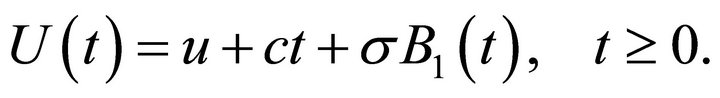
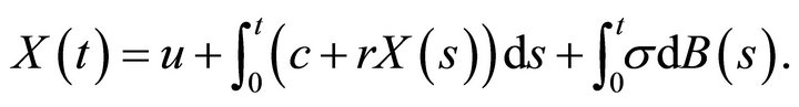
Assume that the insurance business is described by the risk process
 (1.1)
(1.1)
Here,  is the initial capital;
  is the fixed rate of premium income;
  is a standard Brownian motion; and
  is a constant, representing the diffusion volatility.
Suppose that the insurer is allowed to invest in an asset or investment portfolio. Following Paulsen and Gjessing [1], we model the stochastic return as a Brownian motion with positive drift. Specifically, the return on the investment generating process is
 (1.2)
(1.2)
where r and  are positive constants. In (1.2), r is a fixed interest rate;
  is another standard Brownian motion independent of
 , standing for the uncertainty associated with the return on investments at time
 .
.
Let the risk process  denote the surplus of the insurer at time
  under this investments assumption. Thus,
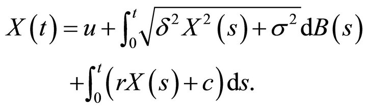
  associated with (1.1) and (1.2) is then the solution of the following linear stochastic integral equation:
 (1.3)
(1.3)
By Paulsen [2] the solution of (1.3) is given by
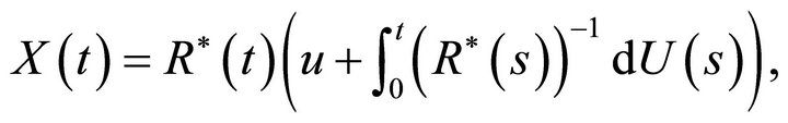 (1.4)
(1.4)
where
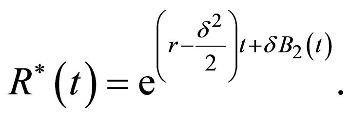
Note that  is a homogeneous strong Markov process, see e.g. Paulsen and Gjessing [1].
The risk process (1.4) can be rewritten as

Because the quadratic variational processes of
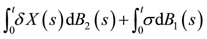
and

are the same, where  is a standard Brownian motion, by Ikeda and Watanabe [3, p. 185] they have the same distribution. Thus, in distribution, we have
 (1.5)
(1.5)
There are many papers concerning occupation times for different risk models. For example, for the classical surplus process with positive safety loading, Egdio dos Reis [4] derived the moment generating function of the total duration of the negative surplus by martingale methods, which was extended in Zhang and Wu [5] to the classical surplus process perturbed by diffusion. Chiu and Yin [6] derived explicit formula for the double Laplace-Stieltjes Transform (LST) of the occupation time in the exponential case for the compound Poisson model with a constant interest. He et al. [7] gived the LST of the total duration of negative surplus for the classical risk model with debit interest. More recently, Wang and He [8] considered the Brownian motion risk model with interest and derived the LST of total duration of negative surplus. In this paper, we consider a Brownian motion risk model with stochastic return on investments. We will use the limitation idea to obtain the LST of total duration of negative surplus.
The remainder of the paper is organized as follows. In Section 2, we give some preliminary results. In Section 3, by exploiting the limitation idea together with the results obtained in Section 2, we obtain the LST of the total duration of negative surplus. In the last section, we present two examples.
2. Preliminary Results
Given , where
 , define
 and if the set is empty
 ,
,
 and if the set is empty
 ,
,
 and if the set is empty
 ,
,
 .
.
Lemma 2.1 The risk process (1.5) has the strong Markov property: for any finite stopping time T the regular conditional expectation of  given
given  is
is
 , that is

where  is the information about the process up to time
 , and the equality holds almost surely.
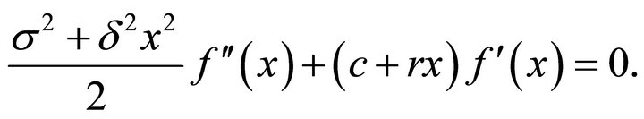
Lemma 2.2 For , the following ordinary differential equation
 (2.1)
(2.1)
has two independent solutions
 (2.2)
(2.2)
and
 (2.3)
(2.3)
where

Proof. From Example 2.2 of Paulsen and Gjessing [1], we get the result.
Lemma 2.3 For ,
,  and
and  ,
,  , define
then
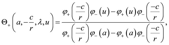

where  and
and  are given by (2.2) and (2.3).
Proof. The result can be found in Chapter 16 of Breiman [9].
Lemma 2.4 For any , then
 (2.4)
(2.4)
where 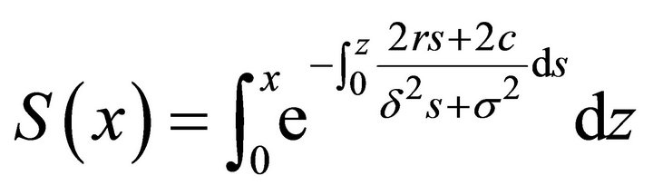 is a solution of the equation
Proof. By Dynkin’s formula,

where  is the generator of diffusion (1.5). It follows that
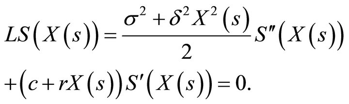
Therefore
Since  is finite, it takes values
  with probability
  and
and  with the complimentary probability. Letting
 , we can assert, by dominated convergence, that
Expanding the expectation on the left, we have
This, together with , gives the result (2.4).
Lemma 2.5 For , the ruin probability for the risk model (1.5) is given by
 (2.5)
(2.5)
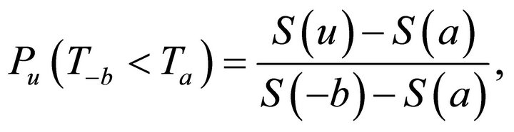
The probability that the surplus process  hit the level
  is given by
 (2.6)
(2.6)
where

Proof. By Lemma 2.4, one can derive (2.5) and (2.6).
3. Total Duration of Negative Surplus
In this section, we will derive the main result of this paper. We assume that the risk process (1.5) does not attain the critical level . For convenience, we assume that the initial surplus
  is positive.
Let the total duration of negative surplus be
For , define two sequences of stopping times of the process (1.5):
 (
( if the set is empty),
( if the set is empty)in general, for
  recursively define
 (
( if the set is empty),

( if the set is empty).
Let . Given
  for some
 , from the strong Markov property of the surplus process, we obtain that the periods
  are mutually independent and have a common distribution. Let
  denote the number of
 .
.
Set . By the monotone convergence theorem, we have
 (3.1)
(3.1)
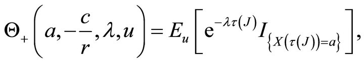
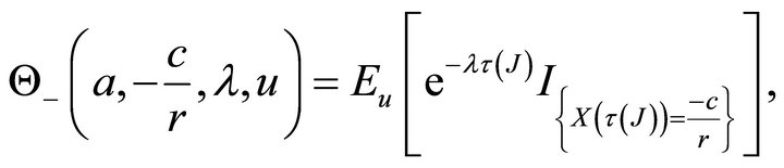
First we give the expression for 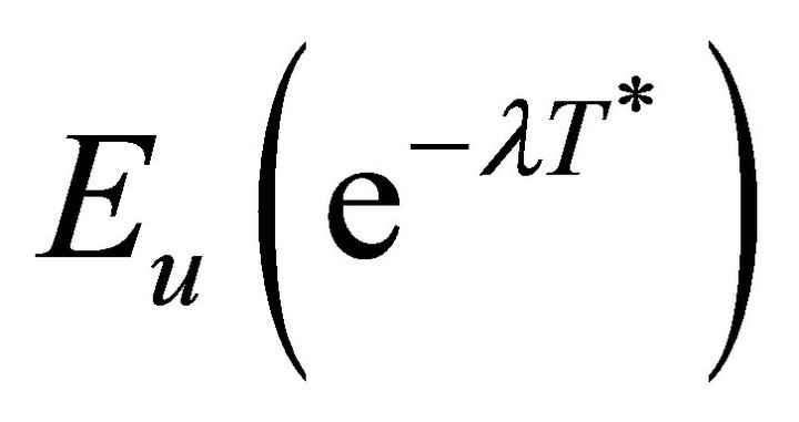 in the following Theorem 3.1.
Theorem 3.1 For  and
and , the LST of
  is given by
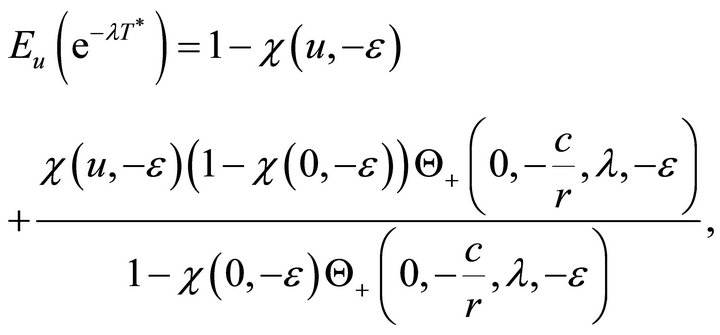 (3.2)
(3.2)
where  and
and  are given by Lemmas 2.3 and 2.5.
Proof. From Lemma 2.1, we can get
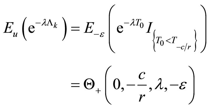 (3.3)
(3.3)
and
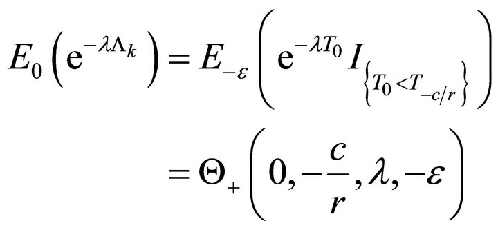 (3.4)
(3.4)
From strong Markov property of the surplus process, we get
This, together with (3.3) and (3.4), gives (3.2).
Theorem 3.2 For  and
and , the LST of total duration of negative surplus is given by
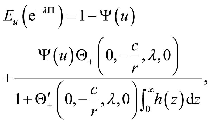 (3.5)
(3.5)
where ,
,  and
and  are given by Lemmas 2.3 and 2.5.
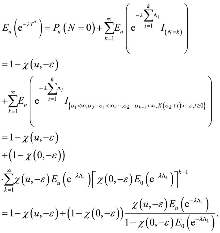
Proof. It follows from (3.1) and (3.2) that
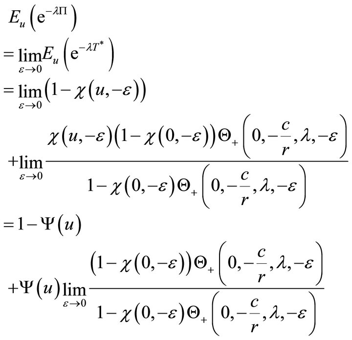 (3.6)
(3.6)
From Lemma 2.5, it follows that
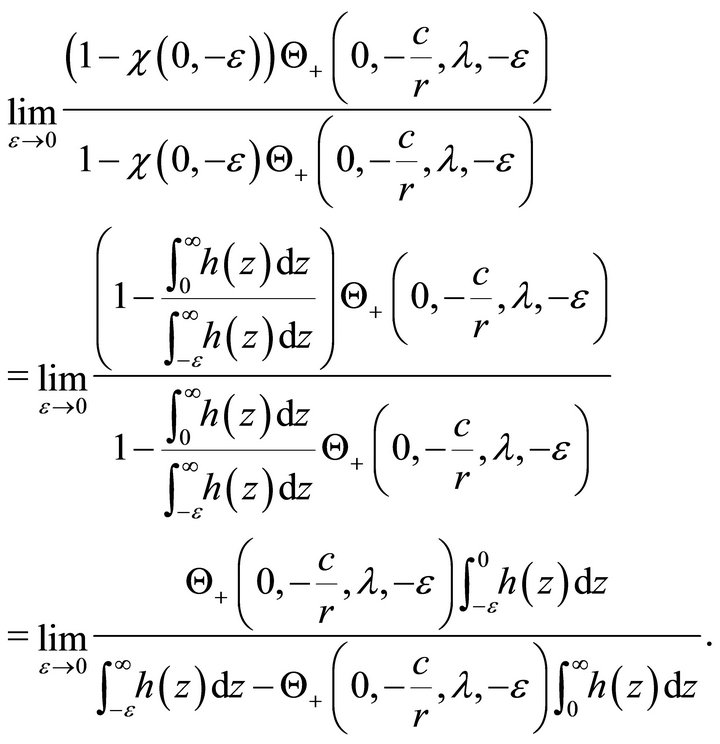 (3.7)
(3.7)
By  Hospital’s rule, we get
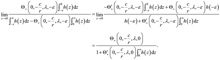
This, together with (3.6) and (3.7), gives (3.5).
4. Examples
In this section we consider two examples.
Example 4.1. Letting  in (1.5), we get the risk model
 (4.1)
(4.1)
From Cai et al. [10], we know that the two independent solutions of the differential equation

are
 (4.2)
(4.2)
and
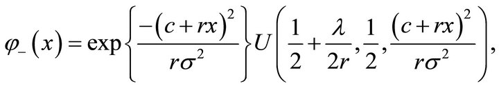 (4.3)
(4.3)
where M and U are called the confluent hypergeometric functions of the first and second kind respectively. More detail on confluent hypergeometric functions can be found in Abramowitz and Stegun [11].
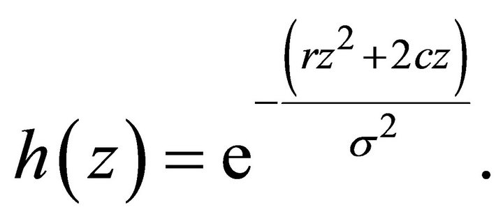
By Lemmas 2.3 and 2.5, we get
 (4.4)
(4.4)
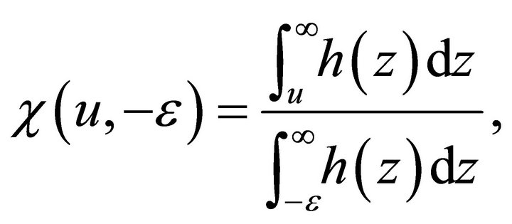 (4.5)
(4.5)
 (4.6)
(4.6)
where
According to Theorems 3.1 and 3.2, we get
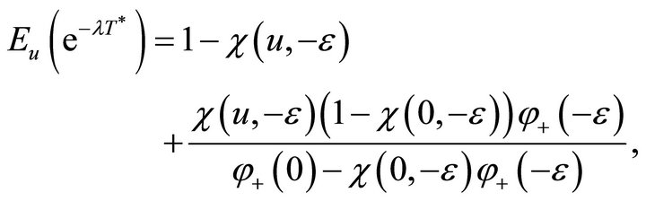 (4.7)
(4.7)
 (4.8)
(4.8)
where ,
,  and
and  are given by (4.2), (4.5) and (4.6).
Remark 4.1 The results (4.7) and (4.8) coincide with the main results in Wang and He [7].
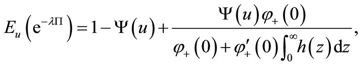
Example 4.2. Letting  and
and  in (1.5), we get the risk model
 (4.9)
(4.9)
It is easy to obtain that the two independent solutions of the ordinary differential equation
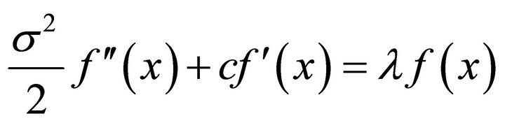
are
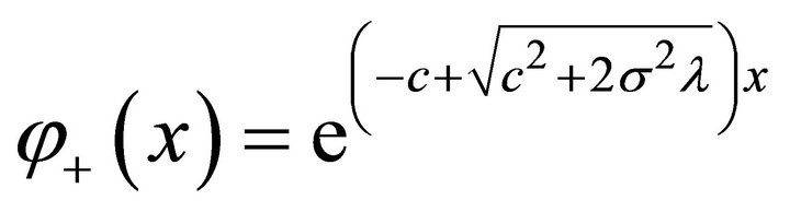
and

By Lemmas 2.3 and 2.5, we get
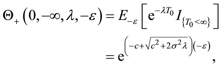

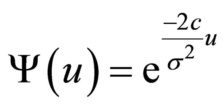
and

According to Theorems 3.1 and 3.2, we have
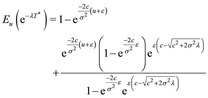
and

5. Conclusion
In this paper, we have studied the diffusion model incorporating stochastic return on investments. We find the LST of the total duration of negative surplus of this process. However, if the risk model (1.1) is extended to a compound Poisson surplus process perturbed by a diffusion, it is difficult to make out. We leave this problem for further research.
REFERENCES
- J. Paulsen and H. K. Gjessing, “Optimal Choice of Dividend Barriers for a Risk Process with Stochastic Return on Investments,” Insurance: Mathematics and Economics, Vol. 20, No. 3, 1997, pp. 215-223. doi:10.1016/S0167-6687(97)00011-5
- J. Paulsen, “Risk Theory in a Stochastic Economic Environment,” Stochastic Processes and Their Applications, Vol. 46, No. 2, 1993, pp. 327-361. doi:10.1016/0304-4149(93)90010-2
- N. Ikeda and S. Watanabe, “Stochastic Differential Equations and Diffusion Processes,” North-Holland Publishing Company, Amsterdam, 1981.
- A. D. Egdio dos Reis, “How Long Is the Surplus below Zero?” Insurance: Mathematics and Economics, Vol. 12, No. 1, 1993, pp. 23-38. doi:10.1016/0167-6687(93)90996-3
- C. S. Zhang and R. Wu, “Total Duration of Negative Surplus for the Compound Poisson Process That Is Perturbed by Diffusion,” Insurance: Mathematics and Economics, Vol. 39, No. 3, 2002, pp. 517-532.
- S. N. Chiu and C. C. Yin, “On Occupation Times for a Risk Process with Reserve-Dependent Premium,” Stochastic Models, Vol. 18, No. 2, 2001, pp. 245-255. doi:10.1081/STM-120004466
- J. M. He, R. Wu and H. Y. Zhang, “Total Duration of Negative Surplus for the Risk Model with Debit Interest,” Statistics and Probability Letters, Vol. 79, No. 10, 2009, pp. 1320-1326. doi:10.1016/j.spl.2009.02.005
- W. Wang and J. M. He, “Total Duration of Negative Surplus for a Brownian Motion Risk Model with Interest,” Acta Mathematica Sinica, 2012, (Submitted).
- L. Breiman, “Probability,” Addison-Wesley, Reading, 1968.
- J. Cai, H. U. Gerber and H. L. Yang, “Optimal Dividends in an Ornstein-Uhlenbeck Type Model with Credit and Debit Interest,” North American Actuarial Journal, Vol. 10, No. 2, 2006, pp. 94-119.
- M. Abramowitz and I. A. Stegun, “Handbook of Mathematical Functions: With Formulas, Graphs, and Mathematical Tables United States Department of Commerce,” US Government Printing Office, Washington DC, 1972.