Applied Mathematics
Vol.3 No.9(2012), Article ID:23012,6 pages DOI:10.4236/am.2012.39155
Parametric Iteration Method for Solving Linear Optimal Control Problems
1Department of Mathematics, Payame Noor University, Tehran, Iran
2Department of Mathematics, Payame Noor University, Mashhad, Iran
Email: alavi601@yahoo.com, a_heidari@pnu.ac.ir
Received June 13, 2012; revised August 7, 2012; accepted August 14, 2012
Keywords: Parametric Iteration Method; Optimal Control Problem; Pontryagin’s Maximum Principle; He’s Variational Iteration Method
ABSTRACT
This article presents the Parametric Iteration Method (PIM) for finding optimal control and its corresponding trajectory of linear systems. Without any discretization or transformation, PIM provides a sequence of functions which converges to the exact solution of problem. Our emphasis will be on an auxiliary parameter which directly affects on the rate of convergence. Comparison of PIM and the Variational Iteration Method (VIM) is given to show the preference of PIM over VIM. Numerical results are given for several test examples to demonstrate the applicability and efficiency of the method.
1. Introduction
Consider linear system described by
 (1)
(1)
where  are the state and control vector, respectively.
  are constant matrix and
  is the initial state. The Optimal Control Problem (OCP) is to find a control law
  which minimizes the quadratic cost functional
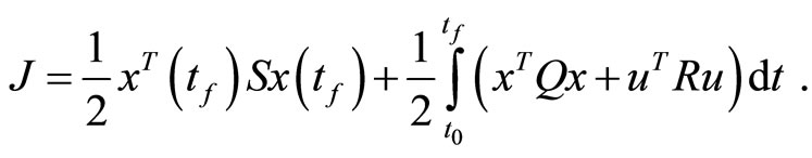 (2)
(2)
where 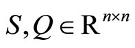 are symmetric positive semi-definite matrices and
 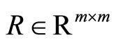 is symmetric positive definite matrix.
In general the problem can be transformed to the Riccati differential equation [1], although solving the Riccati equation arised from OCP is not very simple. Another proposal for directly solving the OCP is discretizing the original problem and solving it numerically. Herein, the spectral collocation methods differ from other computational methods in their special discretization at carefully selected nodes for example, the so-called LegendreGauss-Lobatto nodes. Then the differential equations of the OCP are approximated by algebraic equations [2]. Although these methods are flexible and for programming with computer are compatible, but they have their weaknesses for instance they react quite sensitively on the selection of time-step size [3].
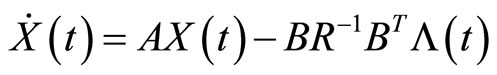
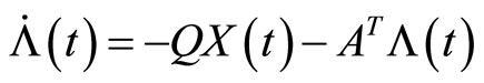
According to the classic optimal control theory, as pointed out in [4], by using Pontryagin’s maximum principle, we can obtain the following Two-Point Boundary Value (TPBV) problem
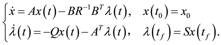 (3)
(3)
and the optimal control law for OCP can be written as  where
where  is known as the costate variable.
Analytic solutions can rarely be found for such TPBV problem and authors often solve it approximately for example Yousefi, Dehghan and Tatari [5] applied He’s Variational Iteration Method (VIM) to find the optimal solutions. In this paper, we are going to solve (3) by use of the Parametric Iteration Method (PIM) with emphasis on preference of PIM over VIM.
2. Parametric Iteration Method
PIM is an approximation method for solving linear and nonlinear problems and at beginning it was proposed for solving nonlinear fractional differential equations [6], by modifying He’s variational iteration method [7]. The idea of PIM is very simple and straightforward. Consider the following differential equation:
 (4)
(4)
where A is a nonlinear operator, t denotes the time, and  is an unknown variable. To explain the basic idea of PIM, we first consider Equation (4) as below:
 (5)
(5)
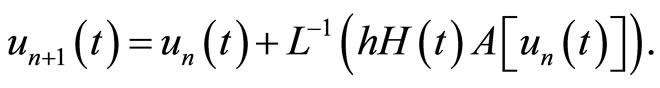
where L denotes a linear differential operator with respect to u, N is a nonlinear operator with respect to u and  is the source term. We then construct a family of iterative formulas as:
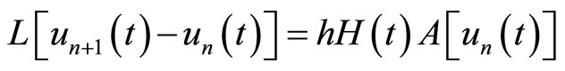 (6)
(6)
where  and
and  denote the so-called auxiliary parameter and auxiliary function respectively. Now by use of
  which is a weighted integral operator, we have:
Accordingly, the successive approximations ,
,  will be readily obtained by choosing the zeroth component
  satisfying the general property
 (7)
(7)
One logical guess for  can be stablished by solving its corresponding linear homogeneous equation
 . Another choice is
  according to the initial condition. Otherwise it can be freely chosen with possible unknown constants. Note that choosing
  can affect on the form of the solutions.
The auxiliary parameter h is an accelerating factor which can be identified optimally by the technique proposed in this paper. We show that a suitable value of h, directly improves the rate of convergence. The auxiliary function  prepare us to have various basis functions to change the solution terms to a desired form. Relation (6) shows that the sequence constructed by PIM is dependent on h and
 , and this directly ables us to identify and control the domain and rate of convergence and this is the main preference of PIM over VIM.
It should be emphasized that though we have the great freedom to choose the linear operator L, the auxiliary parameter h, the auxiliary function , and the initial approximation
 , which is fundamental to the validity and flexibility of PIM, we can also assume that all of them are properly chosen so that solution of (6) exists, as will be shown in this paper later.
Finally, the exact solution may be obtained by using
 (8)
(8)
3. Solution of Optimal Control Problem via PIM
In order to solving the OCP described by (1) and (2), the PIM constructs the following sequences to directly approximate the solutions of the TPBV problem (3),
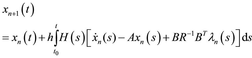 (9)
(9)
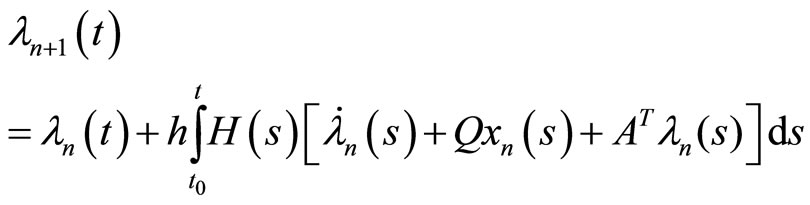 (10)
(10)
Starting with  and
and  as initial approximations,
  and
and  calculate from above iteration formulas. Convergence of these sequences to the optimal solution of the problems (1) and (2) is guaranteed by the following theorem. A similar theorem for nonlinear chaotic Genesio system can be found in [8].
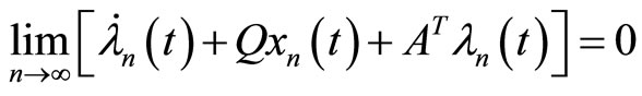
Convergence theorem: if sequence (9) constructed by PIM converges to , then
  is the optimal trajectory of system (1), and if
  is the limit of (10), then the optimal control function
  is
is
Proof: Analytically, as mentioned in [4,5], by having the answers of the system (3), i.e.  and
and , we can establish the optimal control law
  of OCP (1) - (2) and it’s corresponding optimal trajectory
 . Hence if we show that the limits of the iteration formulas (9) and (10) are the answers of the system (3), then the proof is complete. To this end, suppose that
 (11)
(11)
Also consider that  and
and  be uniformly convergent. This hypothesis is in order to guarantee convergence of sequence of derivatives to derivative of the limit i.e.
 (12)
(12)
Now
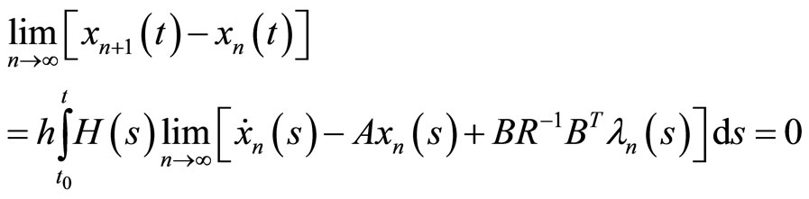
and since , we have:
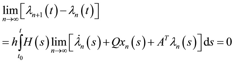
Now by substituting (11) and (12) we have:
Also  and
and  satisfy in conditions of system (3), because:
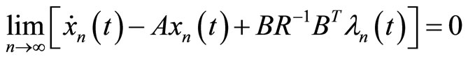
This shows  and
and  are the answers of system (3), and this completes the proof.
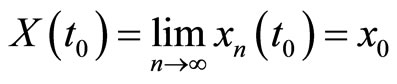
Remark 1. Unfortunately the second condition of system (3) i.e. , is not an initial condition, so the initial approximation for iteration formula (10) is not available. To overcome this difficulty we use a technique likes shooting method, such that first we let
  where s is a constant and calculate
  using (10), next we apply the condition
  and solve this equation due to s as an unknown to find out s. Finally we return to iteration formula (10) with
  as an initial approximation.
Remark 2. Finding an optimal h: h is a parameter in this method which has effect on the rate of convergence. If  this method is coinciding on He’s variational iteration method. But we show by several examples that a suitable value of h, directly improves the rate of convergence. An optimal value of the convergence accelerating parameter h can be determined by the residual error
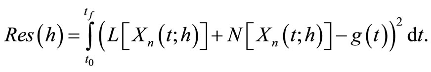 (13)
(13)
One can easily minimize (13) by imposing the requirement .
.
4. Illustrative Examples
In this section, we solve several examples by the PIM to show the efficiency and usefulness of the method indicating on the influence of parameter h on decreasing the iterations and increasing the convergence rate and accuracy of approximations. Whenever the form of approximations has no importance, we take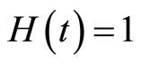 . As pointed out in section 3, we solve OCPs by solving the corresponding TPBV problems (3).
Example 1. Consider the following optimal control system [4]:
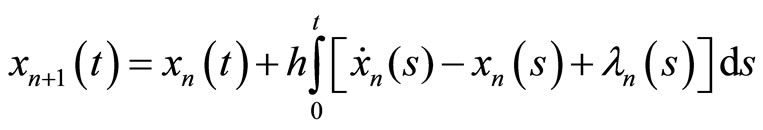
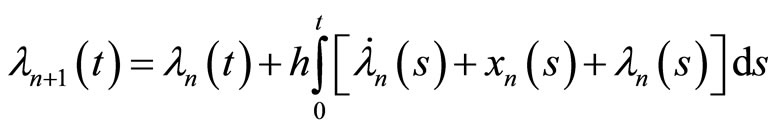
The PIM constructs the following sequences to approximate the solutions:
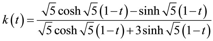
The exact solutions are:
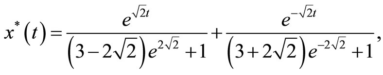
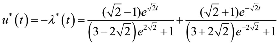
Figure 1, shows the approximate results obtained from the above iteration formulas for n = 2. As shown in figure1 when  approximations are not so good. To improve the accuracy we have to increase iterations, whereas by changing the auxiliary parameter
  we can accelerate the convergence and establish good estimations by lower iterations. This shows the flexibility and excellence of the PIM. Figure 2 is plot of the error for various iterations. It is clear that accuracy of PIM is higher than VIM.
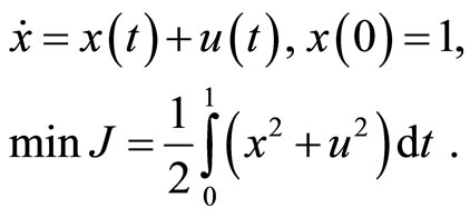
Example 2. Consider the following system:
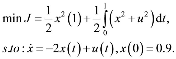
According to [4,5],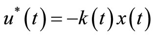 . In Figure 3, the approximate value for
  and its exact value are plotted for
  and optimal value
 . The exact value of
  is
is
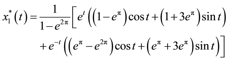
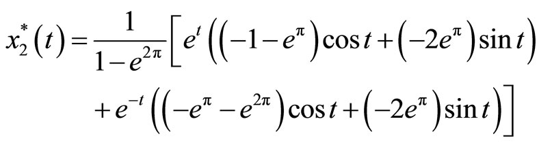
Example 3. Consider a second-order system as follows:
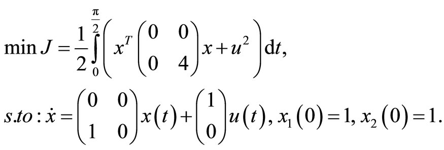
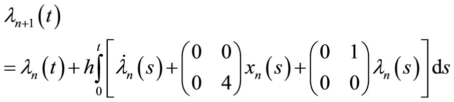
According to Equations (9) and (10), the iteration formulas are:
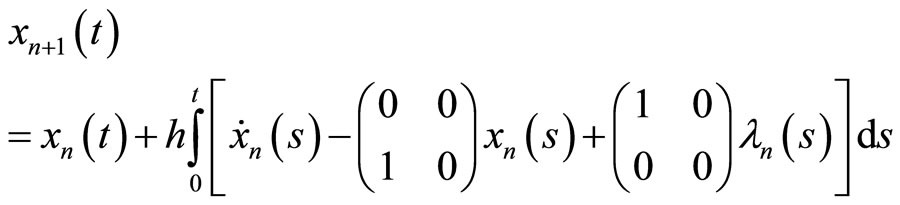
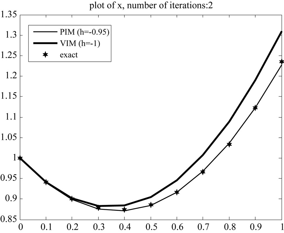
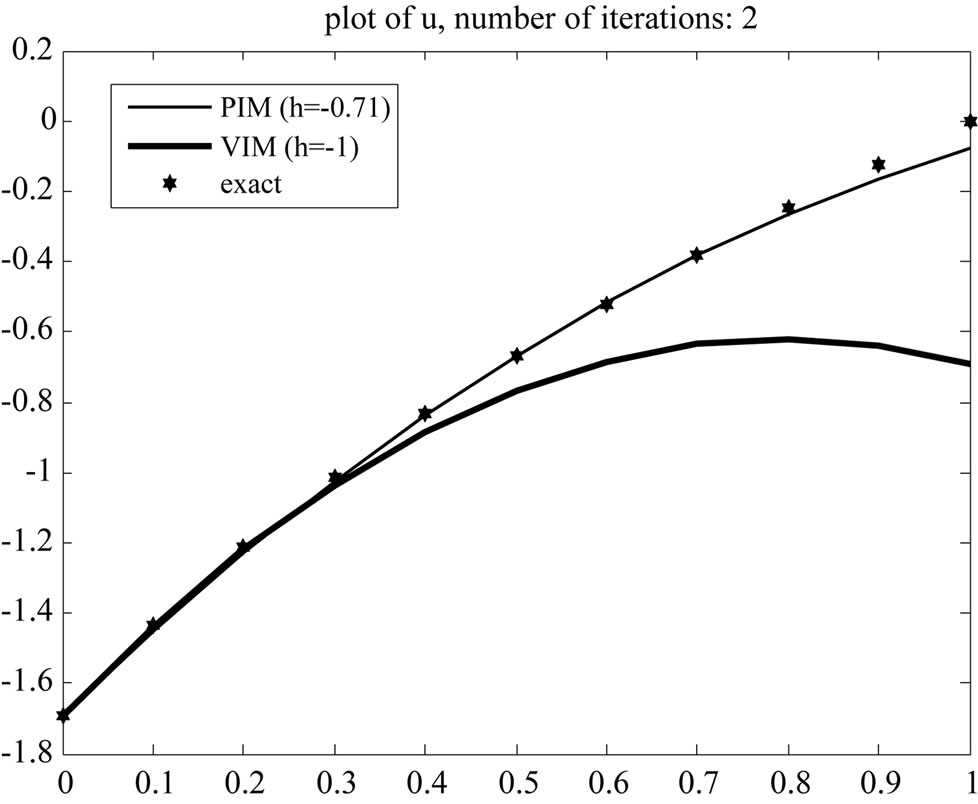
Figure 1. Plot of exact and approximation solutions.
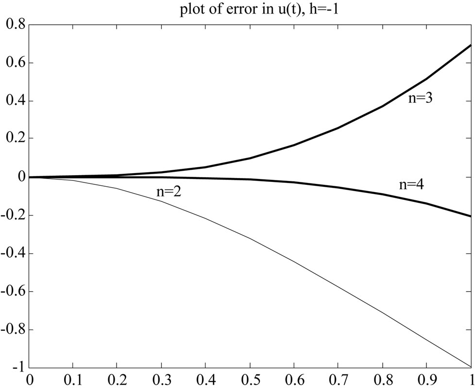
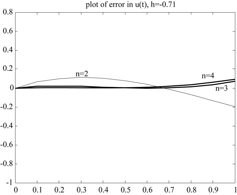
Figure 2. Plot of errors, left: VIM, right: PIM.
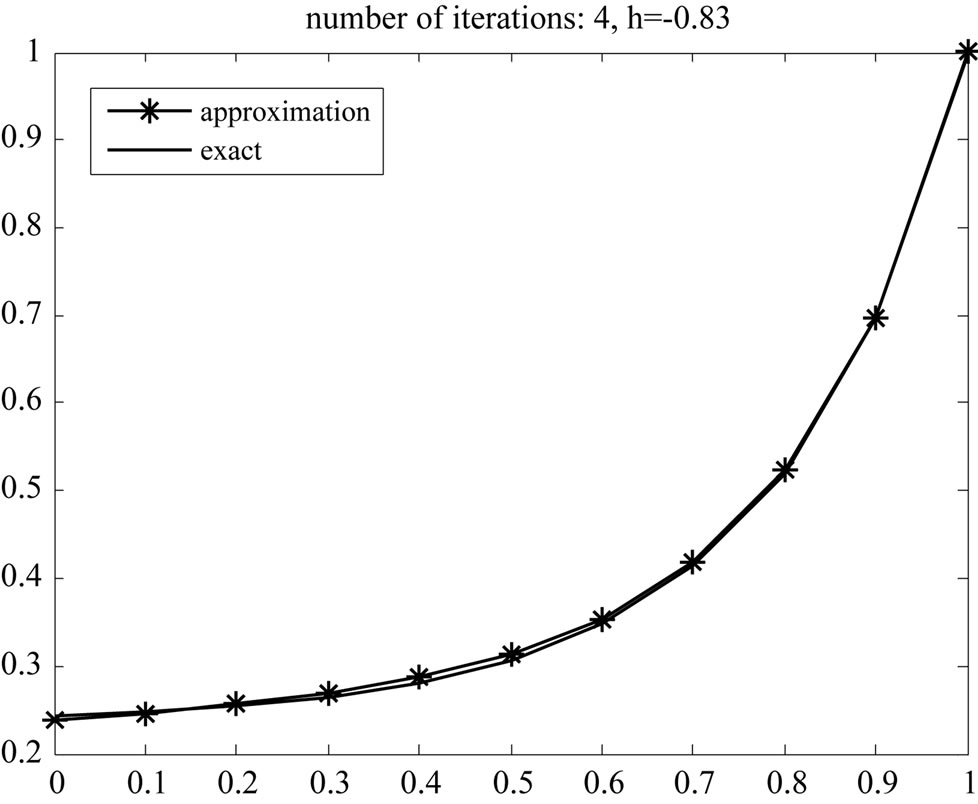
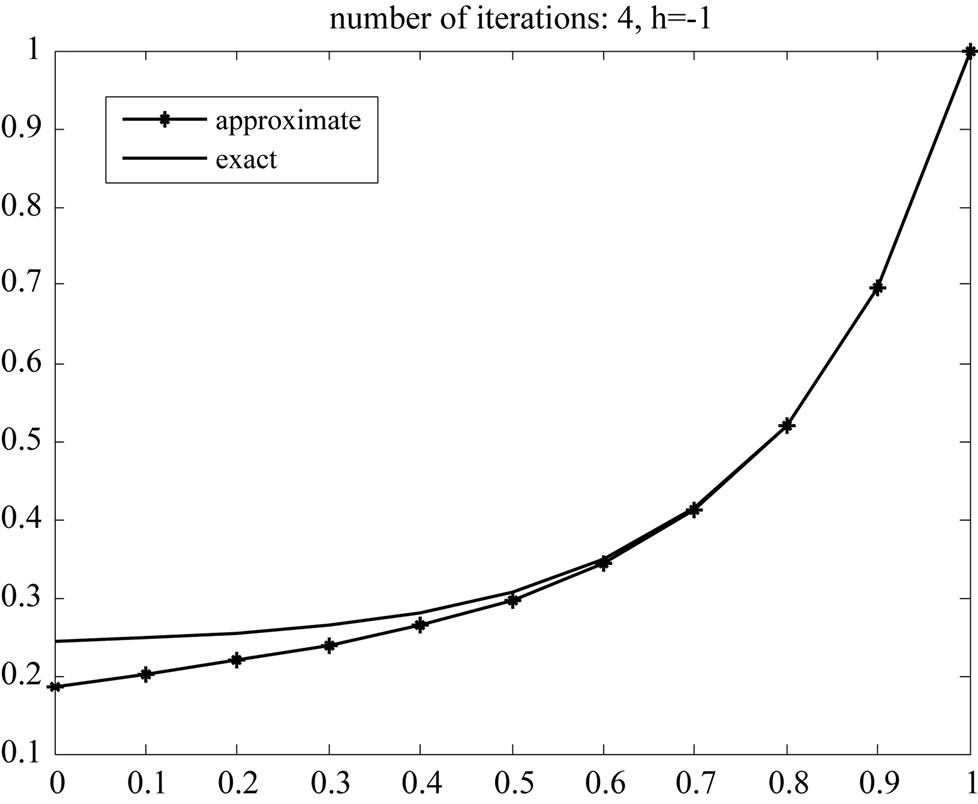
Figure 3. Exact and approximate solution and affection of h.
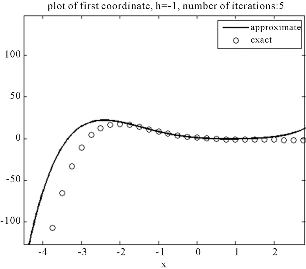
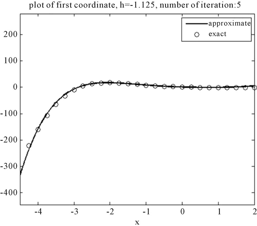
Figure 4. Plot of first coordinate for various h.
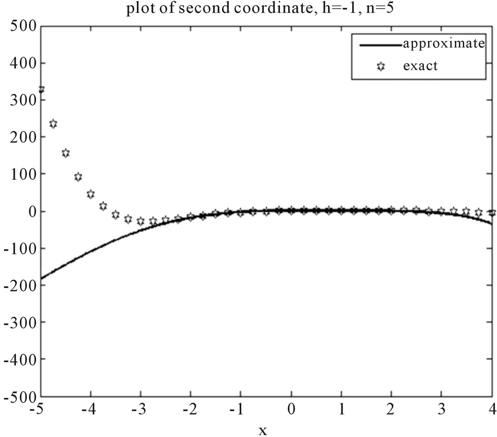
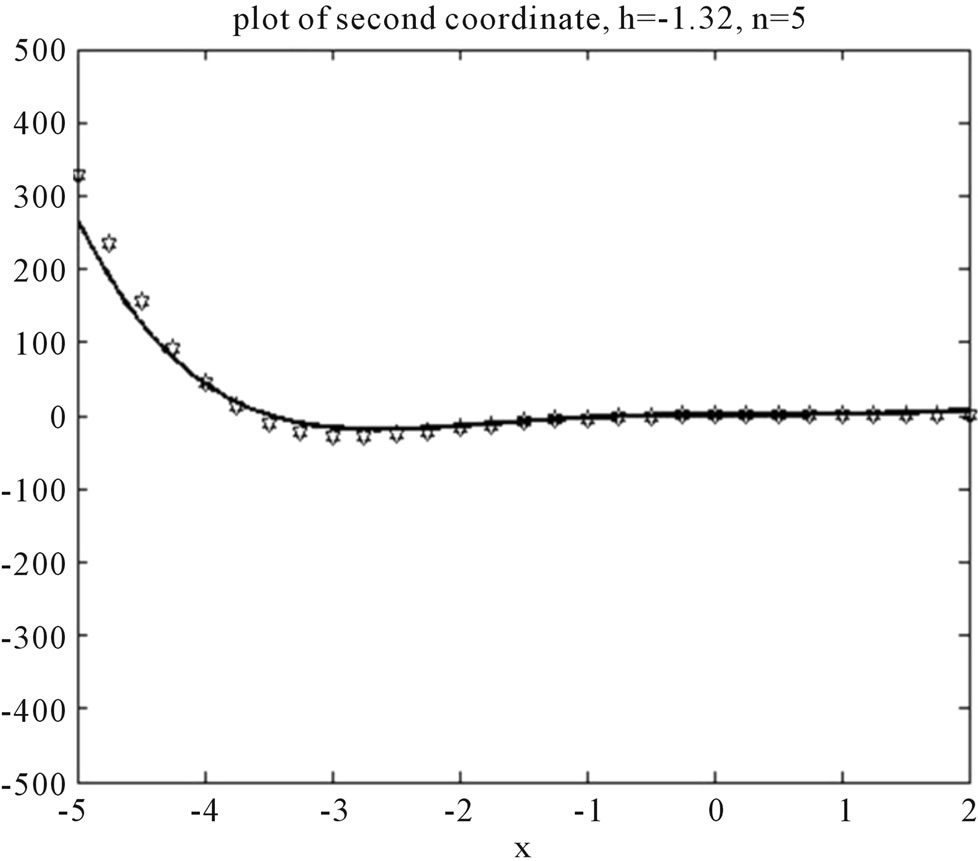
Figure 5. Plot of second coordinate for various h.
The exact solutions are:
Figures 4 and 5 show the exact and approximate solutions. This problem was solved by VIM in [5] and their presented solutions are only in a small region [1.4, 1.7].
5. Conclusion
There are various methods for solving linear OCPs, but in practice, the preferred method is that which be executable by computers and the PIM is one of them, because, moreover it’s simple structure, it has an accelerator parameter h which directly increases the convergence rate and decreases the number of iterations and this ability will be interesting for using in the softwars. One idea to estimate optimal h mentioned in the paper. In general finding optimal auxiliary parameter h and auxiliary function , are open problems. This easy to use method can be used for nonlinear systems too.
REFERENCES
- L. Ntogramatzidis and A. Ferrante, “On the Solution of the Riccati Differential Equation Arising from the LQ Optimal Control Problem,” Systems & Control Letters, Vol. 59, No. 2, 2010, pp. 114-121. doi:10.1016/j.sysconle.2009.12.006
- P. Williams, “A Gauss-Lobatto Quadrature Method for Solving Optimal Control Problems,” ANZIAM Journal, Vol. 47, 2006, pp. C101-C115.
- M. Yamaguti and S. Ushiki, “Chaos in Numerical Analysis of Ordinary Differential Equations,” Physica D: Nonlinear Phenomena, Vol. 3, No. 3, 1981, pp. 618-626. doi:10.1016/0167-2789(81)90044-0
- C. K. Chui and G. Chen, “Linear Systems and Optimal Control,” Springer-Verlag, Berlin, Heidelberg, 1989. doi:10.1007/978-3-642-61312-8
- S. A. Yousefi, M. Dehghan and A. Lotfi, “Finding the Optimal Control of Linear Systems via He’s Variational Iteration Method,” International Journal of Computer and Mathematics, 2009.
- A. Ghorbani, “Toward a New Analytical Method for Solving Nonlinear Fractional Differential Equations,” Computer Methods in Applied Mechanics and Engineering, Vol. 197, No. 49-50, 2008, pp. 4173-4179. doi:10.1016/j.cma.2008.04.015
- J. H. He, “Variational Iteration Method—A Kind of Nonlinear Analytical Technique: Some Examples,” International Journal of Non-Linear Mechanics, Vol. 34, 1999, pp. 699-708.
- A. Ghorbani and J. S. Nadjafi, “A Piecewise-Spectral Parametric Iteration Method for Solving the Nonlinear Chaotic Genesio System,” Mathematical and Computer Modeling, Vol. 54, No. 1-2, 2011, pp. 131-139. doi:10.1016/j.mcm.2011.01.044