Applied Mathematics
Vol. 3 No. 5 (2012) , Article ID: 19064 , 10 pages DOI:10.4236/am.2012.35074
Computation of the Multivariate Normal Integral over a Complex Subspace
1Abdul Salam School of Mathematical Sciences, GC University, Lahore, Pakistan 2Vekua Institute of Applied Mathematics, Tbilisi State University, Tbilisi, Georgia
3Air University Multan Campus, Multan, Pakistan
Email: kartlos55@yahoo.com, muntazimabbas@gmail.com
Received January 25, 2012; revised March 30, 2012; accepted April 6, 2012
Keywords: Multivariate Normal Integral; Random Variable; Probability; Moments; Series
ABSTRACT
The computation of the multivariate normal integral over a Complex Subspace is a challenge, especially when the integration region is of a complex nature. Such integrals are met with, for example, in the generalized Neyman-Pearson criterion, conditional Bayesian problems of testing many hypotheses and so on. The Monte-Carlo methods could be used for their computation, but at increasing dimensionality of the integral the computation time increases unjustifiedly. Therefore a method of computation of such integrals by series after reduction of dimensionality to one without information loss is offered below. The calculation results are given.
1. Introduction
At testing many hypotheses with reference to the parameters of multivariate normal distribution, the problem of computation of multivariate normal integrals over a Complex Subspace of the following form arises [1]
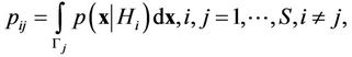 (1)
(1)
where  is the number of tested hypotheses
  supposing that sample
 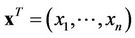 was brought about by distribution

where 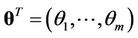 is the vector of distribution parameters and
  is the acceptance region of hypothesis
  from sample space
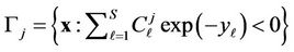
 , which has the following form
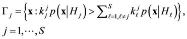 (2)
(2)
where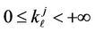 ,
, .
.
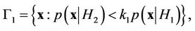
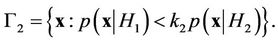
Such regions of hypotheses acceptance arise, for example, in the generalized Neyman-Pearson criterion, and also in conditional Bayesian problems of testing many hypotheses [2,3]. The dimensionality of these integrals often reaches several tens when practical problems are solved. For example, in ecological problems the number of controlled parameters, according to which the decision is made, is quite often equal to several tens [4]; in the air defence problems, in particular, in the problems of tracking of flying objects using radar measurement information, the dimensionality of the problem is equal to the multiplication of the number of flying objects by the number of surveys made by the radar set [5] and so on. On the other hand, the time for solution of these problems is often limited and at times it plays a decisive role especially at solving the defence problems.
It is known that the complexity of realization and the obtained accuracy of numerical methods of computation of multidimensional integrals depend heavily on the dimensionality of these integrals and the complexity of the integration region configuration. In the considered case the integration regions are nonconvex and quite complex. Therefore it is difficult to realize the numerical methods and to provide the desired accuracy of calculation even when the dimensionality of integral is greater than or equal to three [6]. The methods of computation of the multivariate normal integral on the hyperrectangle offered in [7-12] are unsuitable for this case because of the complexity of the integration region.
Despite the convenience and the simplicity of computations, the Monte Carlo method is computer time consuming, especially at large dimensionality of integrals [3,13,14]. Therefore the method of approximate computation of integral (1) for a very short period of time is topical in many applications of mathematical statistics [15,16].
The aim of the present paper is the development of the method of computation of probability integral (1) with the desired accuracy in a minimum of time.
2. Problem Statement
Let us consider the case when the probability distribution density of the vector  looks like
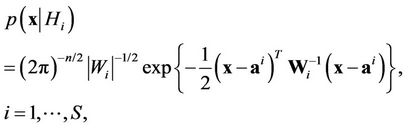 (3)
(3)
where
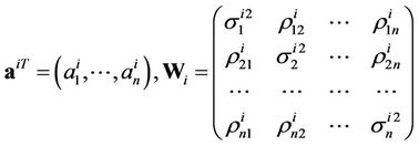 .
.
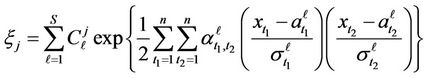
For probability distribution density (3), let us rewrite decision-making region (2) as
 , (4)
, (4)
where
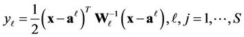 . (5)
. (5)
Random variables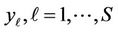 , are squared forms of the normally distributed random vector, and, if hypothesis
  is true, their mathematical expectations are equal to
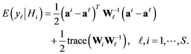 (6)
(6)
Therefore, if hypothesis  is true, the random variable
  has noncentral distribution
  with the degree of freedom
  and with the parameter of noncentrality equal to (6) [2,17,18].
It is obvious that, at  and hypothesis
  is true, the random variable
  has the central
  distribution with the degree of freedom
 .
.
Let us write down (1) as follows
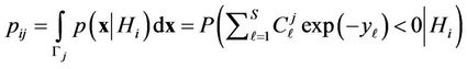 (7)
(7)
The task consists in the computation of probability (7). The method of its analytical computation is not known so far. For its computation it is possible, for example, to use a modified Monte-Carlo method (with the purpose of reducing the computation time) [3]. Though, at large , it still takes a good deal of time. The method of computation of probability (7) if hypotheses are formulated with reference only to the mathematical expectation of normally distributed random vector is offered in [3]. This method is unsuitable here, as the random variable
 (8)
(8)
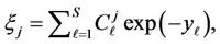
which formulates integration region (4), in [3] is the weighted sum of log-normally distributed random quantities;  and
and  are determined by formulae (5). In our case,
  is the weighted sum of the exponents of negative quadratic forms of the normally distributed random vector with correlated components.
Let us consider the case . In this case, regions (2) take the form
With taking into account probability densities (3), for these regions we derive


where
 .
.
Let us designate
 ,
,
 .
.
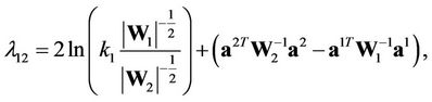
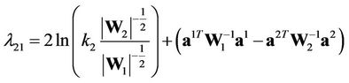
Then, finally, for the required regions, we shall obtain
 .
.
Each of random variables  and
and  is the sum of three random variables one of which is distributed by the normal law, and the two others are distributed by the
  law. Therefore, the probability distribution laws of random variables
  and
and  have not closed forms.
Thus, at , i.e. at testing two hypotheses with respect to all parameters of multivariate normal distribution (in contradistinction to the case when hypotheses are formulated with respect to only the vector of mathematical expectation [3]), the principal complexity of the considered problem does not decrease.
3. Computation of Probability Integral (7) by Series
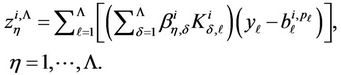
Let us use the expanded form of representation of the quadratic form in (8) [18,19]. Then
 (9)
(9)
where  are the coefficients determined unambiguously by the elements of matrix
  (see formula (3)).
Let  be the conditional density of probability distribution of the random variable
 . Then, for (7), we obtain
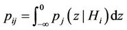 . (10)
Here the infinite interval  is taken as the domain of definition of random variable
  because of the signs of coefficients
  from (5).
As was mentioned above, the probability distribution law of the random variable  has not a closed form. Let us consider the opportunity of approximating this density by series. For this reason we need the moments of the random variable
  [19-21]. Let us consider the problem of obtaining of these moments.
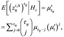
With this purpose let us calculate the initial moment of the  th order of random variable
  provided that hypothesis
  is true
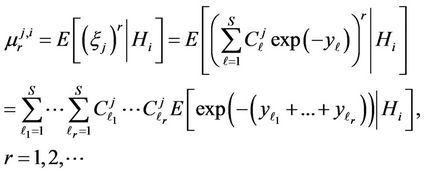 (11)
(11)
Expression  is the sum of correlated Quadratic Forms distributed by noncentral
  probability distribution laws. Because of correlation, the property of reproducibility of the
  distribution does not take place [2,18], and, consequently the mathematical expectation in (12) has not a closed form.
Let us use power series expansion of the exponent
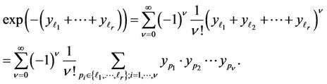 (12)
(12)
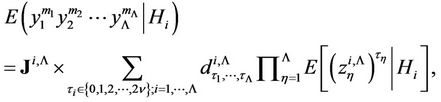
Let us use the expanded representation of quadratic form (9) and be satisfied with the first  terms of expansion (12). Then expression for calculation of moments (11) can be represented as follows
 (13)
(13)
where 
 and
and  .
.
Expression (13) contains product moments [17,19,20] of the  (
( ) orders of normalized components of the correlated normally distributed random observation vector. Therefore, they are not equal to zero [18]. A lot of works are dedicated to the problem of computation of product moments [see, for example, 22-28].
In [22] the following problem was solved. Let  be random variables with mutually independent distributions, and let
 . There is found the probability that
  lies between
  and
and , i.e.
 , by using the central limit theorem in accordance with which the random variable
  is approximately distributed by the normal law. The better is this approximation the bigger is
 .
.
The variance of the product of two random variables was studied by Barnett (1955) and Goodman (1960), in the case when they do not need to be independent. Shellard (1952) studied the case when the distribution of  was (approximately) logarithmic-normal. The author considered the case when
  are random variables with mutually independent distributions. For finding the probability that
  lies between
  and
and  , i.e.
 , the central limit theorem is used to approach the probability distribution of the random variable
  by normal distribution and this approach is better at increasing
 . In work [25] no assumption is made about the distribution of
 . There is discussed the case when the
  random variables,
  ,
,  are mutually independent, and the case when they do not have to be independent, and there are obtained their variance formulae. These results are generalizations of the results presented in [24].
In [26] are given exact formulae for the mathematical expectation of  and
and  ,
,  , where
  is the sample mean of the
  th “character” in a sample of
  elements from a population of
  elements and
  is the corresponding population mean. Formulae for estimating these product moments from the sample were also given. These estimations are slightly biased. In [27] the unbiased estimate of the 4-variate product moment was obtained. Asymptotic results for the 3-variate and 4-variate product moments and their estimates were also obtained.
In [28] is derived a formula for the product moment ,
,  in terms of the joint survival function when
  is a non-negative random vector.
From the given review (of course incomplete, because this is not the aim of this paper) of the works dedicated to the study of product moments, it is seen that the problem considered here differs from them.
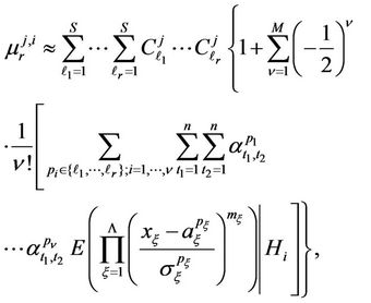
Theorem 3.1. The initial moment of the  th order of random variable
  determined by (9), provided that hypothesis
  is true, can be calculated with any specified accuracy by the formula
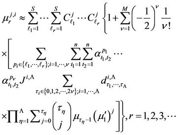 (14)
(14)
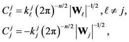
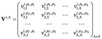
where ;
;  and
and  are the matrices of eigenvectors and eigenvalues of the inverse covariance matrix of normalized random variables
 ;
; ,
, 
 , are the coefficients determined by the terms of matrices
  and
and  and vector
 ;
;  and
and  are the initial and central moments of the first and
  orders, respectively, defined by formulae (22), (23) and (24).
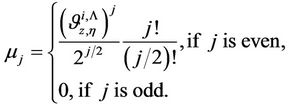
Proof. If hypothesis  is true, the values
 are correlated normally distributed random variables with the parameters
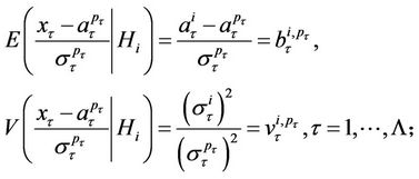
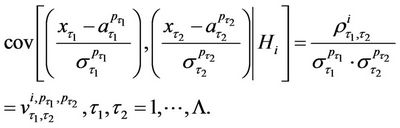 (15)
(15)
Thus, for calculation of moments (13), it is required to calculate the product moments of  -dimensional
  normally distributed random vectors for which the components of the vectors of mathematical expectations and the covariance matrices are calculated by formulae (15).
Let us designate
 ,
,
 , (16)
and the corresponding random vector—by
 , i.e.
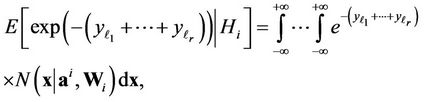
For calculation of conditional product moments of the  -order, we have
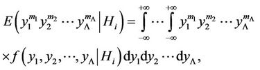 (17)
(17)
where  is the
  -dimensional normal probability distribution density with the vector of mathematical expectations and the covariance matrix calculated by formulae (16).
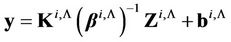
It is known that the value of integral (17) is invariant to linear transformation of the components of vector  [18] with the accuracy of Jacobian of Transformation. Let us designate the matrixes of eigenvectors and eigenvalues of matrix
  by
by  and
and  , respectively. It should be pointed out that
  is a diagonal matrix. Then the components of
  - dimensional random vector
 , (18)
will be uncorrelated and will have standard normal distribution of probabilities [3,20].
From (18), we write
 .
.
Let us introduce the following designation
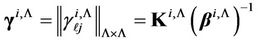 .
.
Then, for the elements of the vector , we obtain the following expression
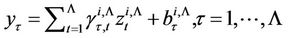 . (19)
Using transformation (19), for mathematical expectation (17), we obtain
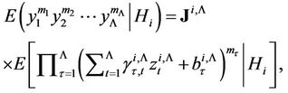 (20)
(20)
where 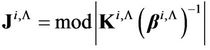 is the Jacobian of Transformation (18).
Let us raise to the powers the linear forms in the righthand side of expression (20) and group the identical items. Then (20) can be written as
 (21)
(21)
where, the coefficients of the identical items in (20) are designated by ,
, ; the items of the vector
  are determined as
It is known that [21,29]
 (22)
(22)
where  and
and  are the initial and central moments of
  and
and  orders, respectively, of random variable
 . After simple routine transformations, for the considered case we obtain
 (23)
(23)
Here
 (24)
(24)
Taking advantage of ratios (21), (22), for computation of the moments (13), we obtain expression (14).
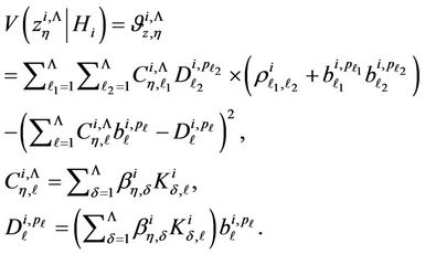
Probability integral (10) can be computed with the help of Edgewort’s series [19-21] using formula (14) for computation of the initial moments of random variable (9). In particular, in the considered case, using wellknown techniques of obtaining Edgewort’s series [30], we have
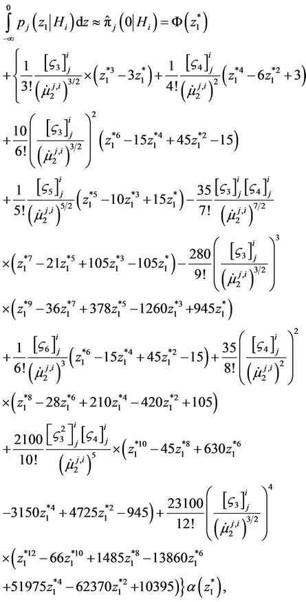 (25)
(25)
where ;
; ,
,  is the
  th semi-invariant of the random variable
  provided hypothesis
  is true (the computation of semi-invariants is not difficult knowing all initial moments includeing
  (see, for example, [21]));
  is the second central moment;
  is standard normal density, i.e.
 .
.
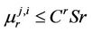
Satisfying the first seven terms in expansion (25), the absolute value of calculation error of the probability integral is calculated by the formula
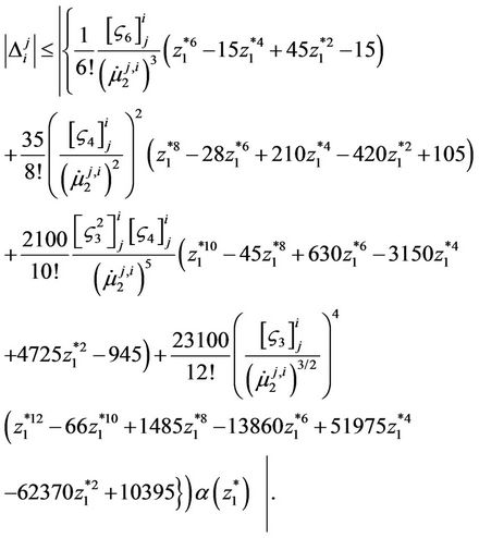
The variable  is continuous and unambiguously defined for every value of
 . Therefore, the random variable
  is continuous. The characteristic function of the random variable
  and its derivatives of any order exist, as the moments of any order of this random variable exist. At the same time, the characteristic function is uniformly continuous. Consequently, the distribution function of this random variable exists and is continuous [21].
Theorem 3.2. The distribution function of random variable  exists and is uniquely determined by moments (14).
Proof. For proving this theorem, it is necessary to show that all moments  exist and the following condition takes place [19,21]
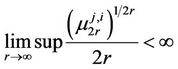 .
.
The fact that all moments exist is obvious from formula (14) as by using it, it is possible to calculate the moments of any order with any specified accuracy. The values of these moments exist and are finite.
When solving the practical problems coefficients  take on the values bounded above; correlation matrices
  are positively determined matrices the determinants of which differ from zero. Therefore, coefficients
  are bounded-above quantities.
There takes place
where  is the sum of quadratic forms of normally distributed
  -dimensional vector
  at different vectors of mathematical expectations and covariance matrices. Therefore, at changing components of the vector
  from
from  up to
up to , the quadratic form
  takes the values from 0 to
 , and the value of function
  varies from 1 to 0, respectively. Therefore [18]
Thus, taking into account (5) and (11) we can write down
where  is the maximum by absolute value among coefficients
 .
.
Assume , then we have
 .
.
Let us designate . Then
 .
.
If , then
  and it is not difficult to be convinced that
  at
at .
.
Let , where
 . Hence
 and
and
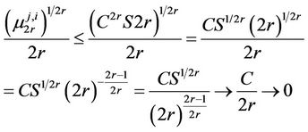
at , which proves the theorem.
4. Computation Results
The accuracy of this algorithm depends heavily on  - the number of used items in expansion (12). In order to increase the accuracy of approximation of the exponent for given
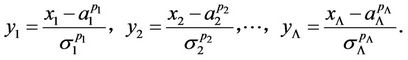
  and, in general, the reliability of computation in the tasks of hypotheses testing, it is expedient to perform first the normalization of initial data by formulae:
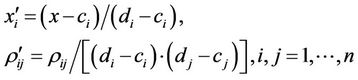
where ,
,  , are the minimum and maximum values of the
  th parameter for the given set of the considered hypotheses, i.e.
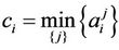 ,
,  ,
,
 ,
,  [3]. In this case, the values of the parameters of the algorithm
  and seven items in expansion (25) provided the absolute error of computation of integral (1) that does not exceed 0.005 for computed examples (see below). This fact was established by modeling for the observation vector with noncorrelated components. Unfortunately, by now the considered algorithm has been realized only for such a case [31].
The results of simulation showed that the time of execution of the task (decision-making and computation of the suitable value of the risk function) by using the Monte-Carlo method made up  sec,
sec,  sec, and
  sec for the number of hypotheses
 ,
,  and
and , respectively, the dimensionality of the observed vector being equal to
  in all cases. The tested hypotheses and correlation matrix for the case
  are given in tables of Figure 1 and Figure 2, respectively. Figures are presented as the suitable forms of the task of hypotheses test of the statistical software in which the appropriate methods are realized [31]. For other values of
 , there are chosen the suitable sub-sets of the tables of these Figures. In the first column of the table of Figure 1 is given the vector of measurements and in the other columns are given hypothetical values of mathematical expectation of this vector.
Meanwhile, when using the method offered here, the computation time did not practically change and the results were obtained for the time noticeably less than 1 sec. In both cases probability integrals (7) were computed with the accuracy of . In Figures 3 and 4 are given the dependences of the integral computation time on the accuracy and number of tested hypotheses respecttively.
At solving many practical problems, especially military problems [5,32], the dimensionality of the integrals
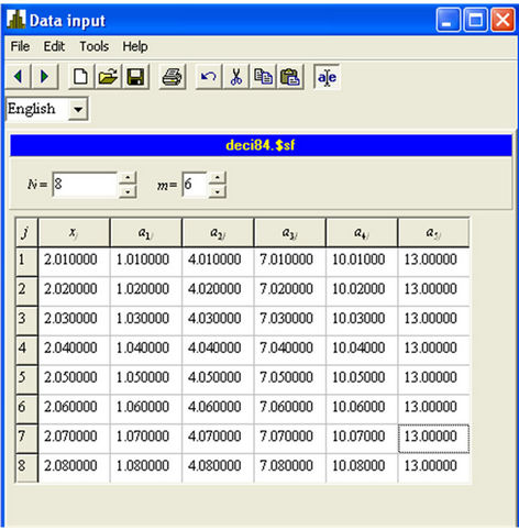
Figure 1. The form of entering the tested hypotheses and a measurement vector.
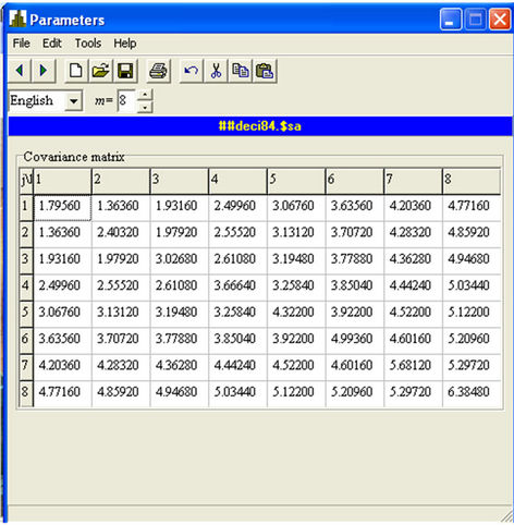
Figure 2. The form of entering the covariance matrix.
like (1) often is equal to several tens and difference between the computation time necessary for the considered methods is significantly longer than in the above mentioned case [14], whereas the computation time for solving the defence problems are of great importance.
The theoretical investigation of the dependence of the accuracy of computation of integral (1) on M-the number of items in expansion (13) is a challenging task. Therefore, at program realization of the offered algorithm and, in general, algorithms of such a kind, it is worthwhile to
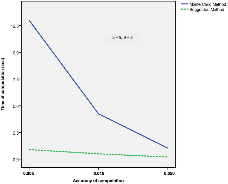
Figure 3. Dependence of the integral computation time on the accuracy.
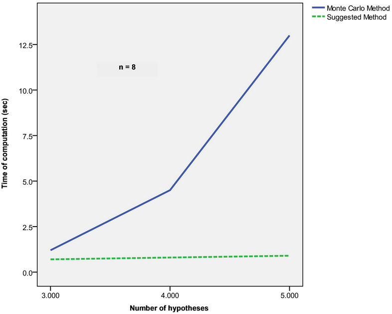
Figure 4. Dependence of the integral computation time on the number of hypotheses.
make parameter  and the number of items in expansion (25) external parameters of the program. This allows establishing their optimal values for each concrete case by experimentation depending on the desired accuracy of computation.
5. Conclusion
The method of computation of the probability integral from the multivariate normal density over the Complex Subspace by using series and the reduction of dimensionality of the multidimensional integral to one without losing the information was developed. The formulae for computation of product moments of normalized normally distributed random variables were also derived. The existence of the probability distribution law of the weighted sum of exponents of negative quadratic forms of the normally distributed random vector was justified. The opportunity of its unambiguous determination by the computed moments was proved.
REFERENCES
- S. Thompson, “On the Distribution of Type II Errors in Hypothesis Testing,” Applied Mathematics, Vol. 2, No. 2, 2011, pp. 189-195. doi:10.4236/am.2011.22021
- C. R. Rao, “Linear Statistical Inference and Its Application,” 2nd Edition, John Wiley & Sons Ltd, New York, 2006.
- K. J. Kachiashvili, “Generalization of Bayesian Rule of Many Simple Hypotheses Testing,” International Journal of Information Technology & Decision Making, Vol. 2, No. 1, 2003, pp. 41-70. doi:10.1142/S0219622003000525
- A. V. Primak, V. V. Kafarov and K. J. Kachiashvili, “System Analysis of Air and Water Quality Control,” Naukova Dumka, Kiev, 1991.
- A. I. Potapov, A. G. Vinogradov, I. A. Goritskyi and E. E. Pertsov, “About Decision-Making of Presence of Objects at Group Measurements,” Questions of Radio-Electronics, Vol. 6, 1975, pp. 69-76.
- P. J. David and P. Rabinovitz, “Methods of Numerical Integration. Computer Science and Applied Mathematics,” 2nd Edition, Academic Press Inc., Orlando, 1984.
- A. Genz, “Numerical Computation of Multivariate Normal Probabilities,” Journal of Computational and Graphical Statistics, Vol. 1, 1992, pp. 141-149.
- A. Genz, “Comparison of Methods for the Computation of Multivariate Normal Probabilities,” Computing Science and Statistics, Vol. 25, 1993, pp. 400-405.
- A. Genz and F. Bretz, “Numerical Computation of Multivariate t-Probabilities with Application to Power Calculation of Multiple Contrasts,” Journal of Statistical Computation and Simulation, Vol. 63, No. 4, 1999, pp. 361- 378. doi:10.1080/00949659908811962
- S. Joe, “Approximations to Multivariate Normal Rectangle Probabilities Based on Conditional Expectations,” Journal of the American Statistical Association, Vol. 90, 1995, pp. 957-964.
- I. H. Sloan and S. Joe, “Lattice Methods for Multiple Integration,” Clarendon Press, Oxford, 1994.
- V. Hajivassiliou, D. McFadden and P. Ruud, “Simulation of Multivariate Normal Rectangle Probabilities and Their Derivatives: Theoretical and Computational Results,” Journal of Econometrics, Vol. 72, No. 1-2, 1996, pp. 85- 134. doi:10.1016/0304-4076(94)01716-6
- J. O. Berger, “Statistical Decision Theory and Bayesian Analysis,” Springer, New York, 1985.
- K. J. Kachiashvili, “Bayesian Algorithms of Many Hypothesis Testing,” Ganatleba, Tbilisi, 1989.
- D. V. Lindley, “The Use of Prior Probability Distributions in Statistical Inference and Decisions,” Proceedings of the 4th Berkeley Symposium on Mathematical Statistics and Probability, Vol. 1, 1961, pp. 453-468.
- L. Tierney and J. B. Kadane, “Accurate Approximations for Posterior Moments and Marginal Densities,” Journal of the American Statistical Association, Vol. 81, 1986, pp. 82-86.
- A. Stuart, J. K. Ord and S. Arnols, “Kendall’s Advanced Theory of Statistics. Classical Inference and the Linear Model,” 6th Edition, Vol. 2A, Oxford University Press Inc., New York, 1999.
- T. W. Anderson, “An introduction to Multivariate Statistical Analysis,” 3rd Edition, Wiley & Sons, Inc., New Jersey, 2003.
- A. Stuart, J. K. Ord and S. Arnols, “Kendall’s Advanced Theory of Statistics. Distribution Theory,” 6th Edition, Vol. 1, Oxford University Press Inc., New York, 1994.
- H. Cramer, “Mathematical Methods of Statistics,” Princeton University Press, Princeton, 1999.
- M. Kendall and A. Stuart, “Distribution Theory,” Vol. 1, Charles Griffit & Company Limited, London, 1966.
- G. D. Shellard, “Estimating the Product of Several Random Variables,” Journal of the American Statistical Association, Vol. 47, 1952, pp. 216-221.
- H. A. R. Barnett, “The Variance of the Product of Two independent Variables and Its Application to an Investigation Based on Sample Data,” Journal of the Institute of Actuaries, Vol. 81, 1955, pp. 190-198.
- L. A. Goodman, “On the Exact Variance of Products,” Journal of the American Statistical Association, Vol. 55, 1960, pp. 708-713.
- L. A. Goodman, “The Variance of the Product of K Random Variables,” Journal of the American Statistical Association, Vol. 57, No. 297, 1962, pp. 54-60.
- S. N. Nath, “On Product Moments from a Finite Universe,” Journal of the American Statistical Association, Vol. 63, No. 322, 1968, pp. 535-541.
- S. N. Nath, “More Results on Product Moments from a Finite Universe,” Journal of the American Statistical Association, Vol. 64, No. 327, 1969, pp. 864-869.
- S. Nadarajah and K. Mitov, “Product Moments of Multivariate Random Vectors,” Communications in Statistics. Theory and Methods, Vol. 32, No. 1, 2003, pp. 47-60. doi:10.1081/STA-120017799
- S. Kotz, N. Balakrishnan and N. L. Johnson, “Continuous Multivariate Distributions. Models and Applications,” Vol. 1, 2nd Edition, John Wiley & Sons Ltd, New York, 2000. doi:10.1002/0471722065
- G. Szego, “Orthogonal Polynomials,” American Mathematical Society, New York, 1959.
- K. J. Kachiashvili and D. I. Melikdzhanian, “SDpro—The Software Package for Statistical Processing of Experimental Information,” International Journal Information Technology & Decision Making, Vol. 9, No 1, 2010, pp. 1-30. doi:10.1142/S0219622010003634
- K. J. Kachiashvili and A. Mueed “Conditional Bayesian Task of Testing Many Hypotheses,” Statistics, 2011, pp. 1-20. doi:10.1080/02331888.2011.602681