Applied Mathematics
Vol. 3 No. 3 (2012) , Article ID: 18109 , 11 pages DOI:10.4236/am.2012.33044
A Measurement Theoretical Foundation of Statistics
Department of Mathematics, Faculty of Science and Technology, Keio University, Yokohama, Japan
Email: ishikawa@math.keio.ac.jp
Received January 6, 2012; revised February 14, 2012; accepted February 21, 2012
Keywords: The Copenhagen Interpretation; Operator Algebra; Quantum and Classical Measurement Theory; Fisher Maximum Likelihood Method; Regression Analysis; Philosophy of Statistics
ABSTRACT
It is a matter of course that Kolmogorov’s probability theory is a very useful mathematical tool for the analysis of statistics. However, this fact never means that statistics is based on Kolmogorov’s probability theory, since it is not guaranteed that mathematics and our world are connected. In order that mathematics asserts some statements concerning our world, a certain theory (so called “world view”) mediates between mathematics and our world. Recently we propose measurement theory (i.e., the theory of the quantum mechanical world view), which is characterized as the linguistic turn of quantum mechanics. In this paper, we assert that statistics is based on measurement theory. And, for example, we show, from the pure theoretical point of view (i.e., from the measurement theoretical point of view), that regression analysis can not be justified without Bayes’ theorem. This may imply that even the conventional classification of (Fisher’s) statistics and Bayesian statistics should be reconsidered.
1. Introduction
For example, consider Newtonian mechanics. It is natural to understand that Newton mechanics is based on Newton’s three laws of motion, though the mathematical theory of differential equations is a useful tool for the analysis of Newtonian mechanics. That is because any mathematical theory is a closed logical system derived from set theory, and thus, it is not qualified to assert statements concerning our world without laws. If it is so, and, if Kolmogorov’s probability theory [1] is a mathematical theory, we think that the foundation of statistics does not yet established. Thus, the following problem is natural:
(A) What kind of law is statistics based on? Or, propose a foundation of statistics!
The purpose of this paper is to answer this problem.
Although in a series of our research [2-8] we have been concerned with this problem (A), in this paper we give a decisive answer to the problem (A) in the light of our final version [7,8] of measurement theory. Here, as mentioned in Section 2 later, measurement theory (i.e., the theory of the quantum mechanical world view) is characterized as the linguistic turn of quantum mechanics. Hence, note that measurement theory is not physics but a kind of language, and thus, the “law” in (A) is called “axiom” in this paper.
2. Measurement Theory (Axioms and Interpretation)
2.1. Mathematical Preparations
In this section, we prepare mathematics, which is used in measurement theory (or in short, MT).
Measurement theory ([2-8]) is, by an analogy of quantum mechanics (or, as a linguistic turn of quantum mechanics), constructed as the scientific theory formulated in a certain  -algebra
  (i.e., a norm closed subalgebra in the operator algebra
  composed of all bounded operators on a Hilbert space H, cf. [9,10]). MT is composed of two theories (i.e., pure measurement theory (or, in short, PMT] and statistical measurement theory (or, in short, SMT). That is, we see:
(B) MT (measurement theory)
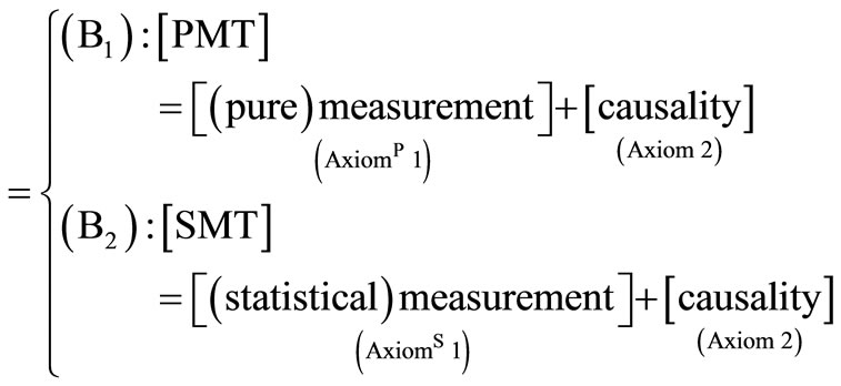
where Axiom 2 is common in PMT and SMT. For completeness, note that measurement theory (B) (i.e., (B1) and (B2)) is a kind of language based on the quantum mechanical world view, (cf. [8]). It may be understandable to consider that
(C) PMT and SMT is related to Fisher’s statistics and Bayesian statistics respectively.
Also, as mentioned in Section 2.6 latter, our concern in this paper is to give an answer to the question “Which is fundamental, PMT or SMT?”.
When , the
, the  -algebra composed of all compact operators on a Hilbert space H, the (B) is called quantum measurement theory (or, quantum system theory), which can be regarded as the linguistic aspect of quantum mechanics. Also, when
  is commutative (that is, when
  is characterized by
 , the
, the  - algebra composed of all continuous complex-valued functions vanishing at infinity on a locally compact Hausdorff space
  (cf. [9])), the (B) is called classical measurement theory. Thus, we have the following classification:
(D) 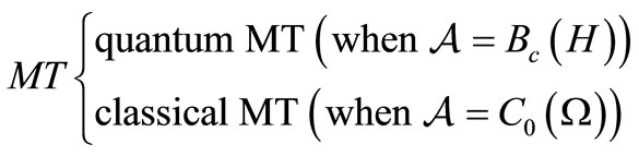
In this paper, we mainly devote ourselves to classical MT (i.e., classical PMT and classical SMT).
Now we shall explain the measurement theory (B). Let  be a
be a  -algebra, and let
  be the dual Banach space of
 . That is,
 {
{ is a continuous linear functional on
  }, and the norm
  is defined by
 .
.
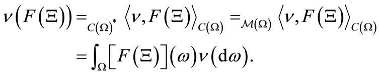
The bi-linear functional  is also denoted by
  , or in short
 . Define the mixed state
  such that
  and
and  for all
  satisfying
 . And put
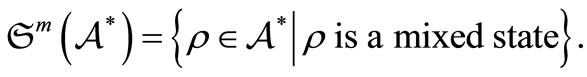
A mixed state  is called a pure state if it satisfies that
  for some
  and
and  implies
 . Put
. Put
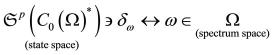
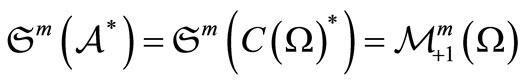
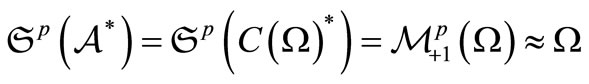
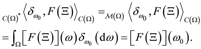
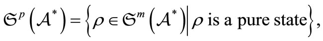 which is called a state space. The Riese theorem (cf. [11]) says that
  ,
,
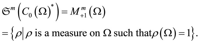
Also, it is well known (cf. [9]) that

and
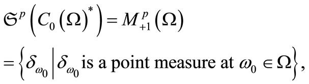
where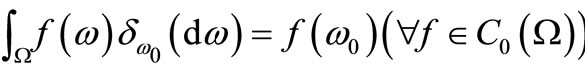 . The latter implies that
  can be also identified with
  (called a spectrum space or maximal ideal space) such as
Here, assume that the  -algebra
  is unital, i.e., it has the identity I. This assumption is not unnatural, since, if
 , it suffices to reconstruct the
  such that it includes
 .
.
According to the noted idea (cf. [12]) in quantum mechanics, an observable  in
in  is defined as follows:
(E1) [Field] X is a set,  (
( , the power set of X) is a field of X, that is, “
 ”, “
”, “ ”.
”.
(E2) [Countably additivity] F is a mapping from  to
to  satisfying: 1) for every
 ,
,  is a nonnegative element in
  such that
 , 2)
, 2)  and
and , where 0 and I is the 0- element and the identity in
  respectively. 3): for any countable decomposition
  of
of  (i.e.,
 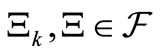 such that
 ,
,  ), it holds that
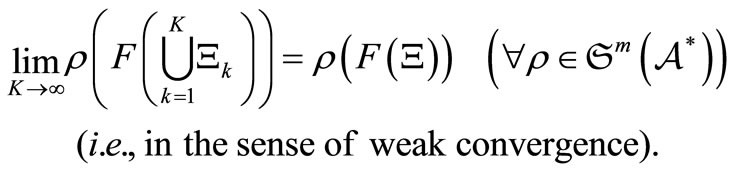 (1)
(1)
Remark 1. By the Hopf extension theorem (cf. [11]), we have the mathematical probability space (X,  ,
,  ) where
  is the smallest
  -field such that
 . For the other formulation (i.e.,
  -algebraic formulation), see the appendix in [7].
2.2. Pure Measurement Theory in (B1)
In what follows, we shall explain PMT in (B1).
With any system S, a  -algebra
  can be associated in which the pure measurement theory (B1) of that system can be formulated. A state of the system S is represented by an element
  and an observable is represented by an observable
  in
in . Also, the measurement of the observable O for the system S with the state
  is denoted by
  (or more precisely,
  ). An observer can obtain a measured value
  by the measurement
  .
.
The AxiomP 1 presented below is a kind of mathematical generalization of Born’s probabilistic interpretation of quantum mechanics. And thus, it is a statement without reality.
AxiomP 1. [Pure Measurement]. The probability that a measured value  obtained by the measurement
  belongs to a set
  is given by
 .
.
Next, we explain Axiom 2 in (B). Let  be a tree, i.e., a partial ordered set such that
  and
and  implies
  or
or . In this paper, we assume that T is finite (cf. Remark 9 in Section 7 later). Assume that there exists an element
 , called the root of T, such that
  (
( ) holds. Put
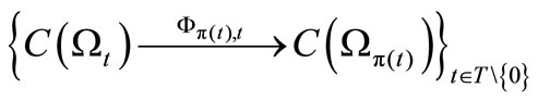
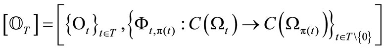
  . The family
  is called a causal relation (due to the Heisenberg picture), if it satisfies the following conditions (F1) and (F2).
(F1) With each , a
, a  -algebra
  is associated.
(F2) For every , a Markov operator
  is defined (i.e.,
  ,
,
 ). And it satisfies that
  holds for any
 ,
, .
.
The family of dual operators  is called a dual causal relation (due to the Schrödinger picture). When
  holds for any
 , the causal relation is said to be deterministic.
Now Axiom 2 in the measurement theory (B) is presented as follows:
Axiom 2. [Causality]. The causality is represented by a causal relation .
.
2.3. Interpretation
Next, we have to study how to use the above axioms as follows. That is, we present the following interpretation (G) [= (G1) – (G3)], which is characterized as a kind of linguistic turn of so-called Copenhagen interpretation (cf. [7,8]). That is, we propose:
(G1) Consider the dualism composed of observer and system (= measuring object). And therefore, observer and system must be absolutely separated.
(G2) Only one measurement is permitted. And thus, the state after a measurement is meaningless since it can not be measured any longer. Also, the causality should be assumed only in the side of system, however, a state never moves. Thus, the Heisenberg picture should be adopted, and thus, the Schrödinger picture should be prohibited.
(G3) Also, the observer does not have the space-time. Thus, the question: “When and where is a measured value obtained?” is out of measurement theory. And thus, Schrödinger’s cat is out of measurement theory, and so on.
2.4. Sequential Causal Observable and Its Realization
For each , consider a measurement
  . However, since the (G2) says that only one measurement is permitted, the measurements
  should be reconsidered in what follows. Under the commutativity condition such that
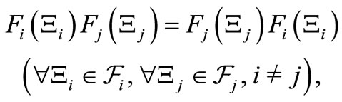 (2)
(2)
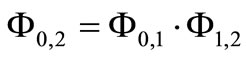
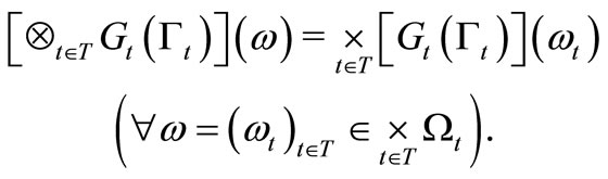
we can define the product observable
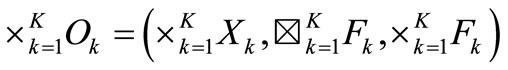 in
in  such that
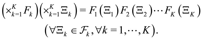
Here,  is the smallest field including the family
 . Then, the above
  is, under the commutativity condition (2), represented by the simultaneous measurement
 .
.
Consider a tree  with the root
 . This is also characterized by the map
 such that
 . Let
. Let  be a causal relation, which is also represented by
 . Let an observable
  in the
  be given for each
 . Note that
  is an observable in the
 .
.
The pair , is called a sequential causal observable. For each
 , put
, put . And define the observable
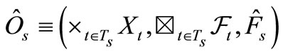 in
in  as follows:
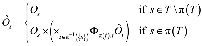 (3)
(3)
if the commutativity condition holds (i.e., if the product observable  exists) for each
  . Using (3) iteratively, we can finally obtain the observable
  in
in . The
. The  is called the realizetion (or, realized causal observable) of
 .
.
2.5. Statistical Measurement Theory in (B2)
We shall introduce the following notation: it is usual to consider that we do not know the pure state
 when we take a measurement
  . That is because we usually take a measurement
  in order to know the state
 . Thus, when we want to emphasize that we do not know the state
 ,
,  is denoted by
 . Also, when we know the distribution
 of the unknown state
 , the
, the
 is denoted by
 . The
. The
 is called a mixed state. And further, if we know that a mixed state
  belongs to a compact set
 , the
, the  is denoted by
 .
.
The AxiomS 1 presented below is a kind of mathematical generalization of AxiomP 1.
AxiomS 1. [Statistical measurement]. The probability that a measured value  obtained by the measurement
  belongs to a set
  is given by
 .
.
Thus, we can propose the statistical measurement theory (B2), in which Axiom 2 and Interpretation (G) are common.
Let  be an observable in a
  - algebra
 . Assume that we know that the measured value
  obtained by a statistical measurement
  belongs to
 . Then, there is a reason to infer that the unknown measured value
  is distributed under the conditional probability
 , where
 (4)
(4)
Thus, by a hint of Fisher’s maximum likelihood method, we have the following theorem, which is the most fundamental in this paper.
Theorem 1. [Fisher’s maximum likelihood method in general ]. Let
  be an observable in a
  -algebra
 . Let
. Let  be a compact set. Assume that we know that the measured value
  obtained by a measurement
  belongs to
 . Then, there is a reason to infer that the unknown measured value
  is distributed under the conditional probability
 , where
 (5)
(5)
Here,  is defined by
Remark 2. Theorem 1 is new throughout our research [2-8], though, in a particular case that , Theorem 1 was proposed in [7] where we devoted ourselves to PMT.
2.6. Our Concern in This Paper
Note that
(H1) 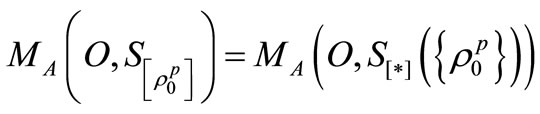 for
for
 , therefore, we see that [PMT]
  [SMT].
However, we have the following problem:
(H2) Which is fundamental, PMT or SMT?
Recalling the (C), most readers may consider that PMT is more fundamental than SMT. In fact, throughout our research [2-8], we have believed in the fundamentality of PMT. However, in this paper, we assert that Theorem 1 in SMT is the most fundamental as far as inference. In fact, every result in this paper is regarded as one of the corollaries of Theorem 1. And hence, we shall conclude that SMT is proper as the answer to the problem (A). Also, our proposal has a merit such that the philosophy of statistics is naturally induced by the philosophy of measurement theory (cf. [8]).
3. Fisher-Bayes Method in Classical 
3.1. Notations
We shall devote ourselves to classical case (i.e.,  ). From here,
  (or, commutative unital
  -algebra that includes
 ) is, for simplicity, denoted by
 . Thus, we put
 ,
,
 and
and
 .
.
And, for any mixed state  and any observable
  in
in , we put:
 (6)
(6)
Also, put  (
( : Borel
  -field). In order to avoid the confusion between
  in (6) and
 , we do not use
 . Also, for any
 , we put:
3.2. Bayes Method in Classical 
Let  be an observable in a commutative
  -algebra
 . And let
  be any observable in
 . Consider the product observable
  in
in . The existence will be shown in Section 7 (Appendix).
Assume that we know that the measured value  obtained by a simultaneous measurement
  belongs to
 . Then, by (4), we can infer that
(I) the probability  that y belongs to
  is given by
Thus, we can assert that:
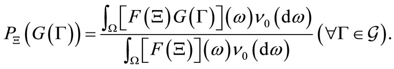
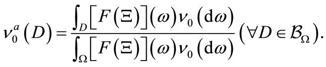
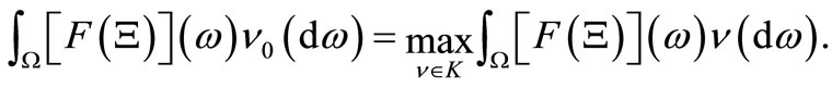
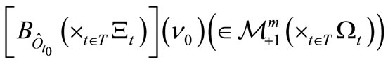
Theorem 2. [Bayes method, cf. [4,5]]. When we know that a measured value obtained by a measurement
  belongs to
 , there is a reason to infer that the mixed state after the measurement is equal to
 , where
Proof. Note that we can regard that
 . That is, there exists
 such that
 (7)
(7)
Then, AxiomS 1 says that the probability that a measured value  obtained by the measurement
  belongs to a set
  is given by
 , which is equal to
  in (7). Since
  is arbitrary, we obtain Theorem 2.
Remark 3. The above (I) is, of course, fundamental. However, in the sense mentioned in the above proof, we admit Theorem 2 as the equivalent statement of the (I). That is, in spite of Interpretation (G2), we admit the wavefunction collapse such as
(J) 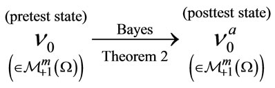
Theorem 2 was, for the first time, proposed in [4,5] without the conscious understanding of Interpretation (G2). Also, note that(K) in Theorem 2, if , then it clearly holds that
 .
.
Also, for our opinion concerning the wavefunction collapse in quantum mechanics, see [7].
3.3. Fisher-Bayes Method in Classical 
Combining Theorem 1 (Fisher’s method) and Theorem 2 (Bayes’ method), we get the following corollary.
Corollary 1. [Fisher-Bayes method (i.e., Regression analysis in a narrow sense)]. When we know that a measured value obtained by a measurement  belongs to
 , there is a reason to infer that the state after the measurement is equal to
  such that
where the  is defined by
Remark 4. As mentioned in the above, note that Corollary 1 is composed of the following two procedure:
(L) 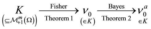
3.4. A Simple Example of Fisher-Bayes Method (Regression Analysis in a Narrow Sense)
In this section, we examine Corollary 1 in a simple example. Readers will find that Corollary 1 can be regarded as regression analysis in a narrow sense.
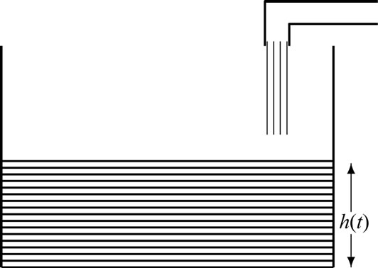
We have a rectangular water tank filled with water. Assume that the height of water at time t is given by the following function :
:
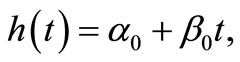 (8)
(8)
where  and
and  are unknown fixed parameters such that
  is the height of water filling the tank at the beginning and
  is the increasing height of water per unit time. The measured height
  of water at time t is assumed to be represented by
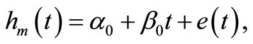 (9)
(9)
where  represents a noise (or more precisely, a measurement error) with some suitable conditions. And assume that we obtained the measured data of the heights of water at
  as follows:
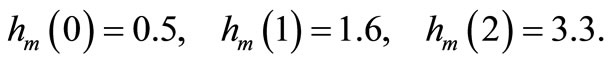 (10)
(10)
Under this setting, we shall study the following problem:
(M) [Inference]: when measured data (10) is obtained, infer the unknown parameter  in (9).
In what follows, from the measurement theoretical point of view, we shall answer the problem (M). Let  be a series ordered set such that the parent map
  is defined by
 .
.
Put ,
,  ,
,
 . For each
 , consider a continuous map
  such that
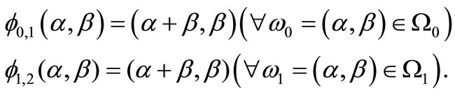 (11)
(11)
Then, we get the deterministic causal operators hus,
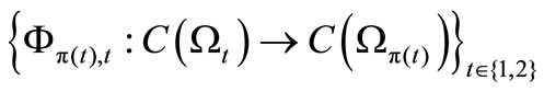 such that
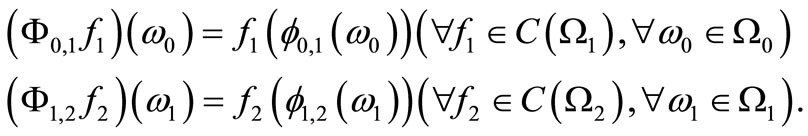 (12)
(12)
Thus, we have the causal relation as follows.

Put ,
, .
.
Let  be the set of real numbers. Fix
 . For each
 , define the normal observable
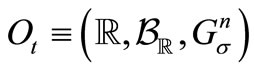 in
in  such that
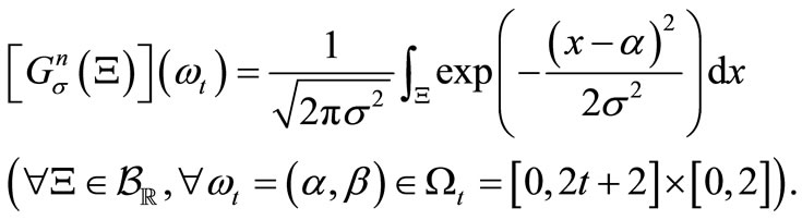 (13)
(13)
Thus, we get the sequential deterministic causal observable
 .
.
Then, the realized causal observable 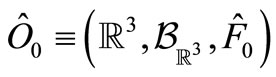 in
in  is, by (3) and (12), obtained as follows:
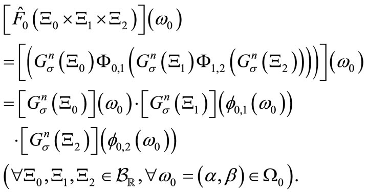 (14)
(14)
Putting , we have the measurement
 . Recall the (10), that is, the measured value
  obtained by the measurement
  is equal to
 (15)
(15)
Define the closed interval  such that
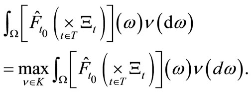
for sufficiently large N. Here, Fisher’s method (Theorem 1) says that it suffices to solve the problem.
(N) Find  such as
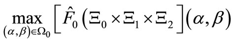 (16)
(16)
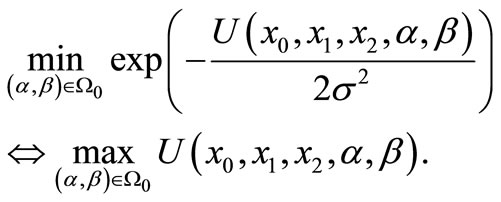
Putting
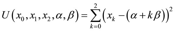
we have the following problem that is equivalent to (N):
(O) Find  such as
Calculating
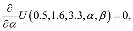
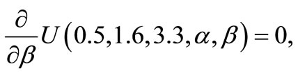
we get
 (17)
(17)
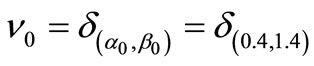
Thus, we see, by the statement (K), that
(P) 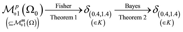
This (i.e., ) is the answer to the problem (M).
Problem 1. Since the above example is quite easy, the validity of Bayes’ theorem in (P) may not be clear. If it is so, instead of the problem (M), we should present the following simple problem.
(Q) Infer the water level at time 1.
Some may calculate and conclude as follows:
 (18)
(18)
However, this calculation is based on the Schrödinger picture, and thus, the justification of this calculation (18) is not assured. That is because measurement theory (particularly, Interpretation (G2)) says that the Heisenberg picture should be adopted. Therefore, in order to answer the problem (Q), we must prepare Corollary 2 (i.e., regression analysis in a wide sense) in the following section.
Remark 5. It should be noted that the following two are equivalent:
(R1) [=(M); Inference]: when measured data (10) is obtained, infer the unknown parameter .
.
(R2) [Control]: Settle the parameter  such that measured data (10) will be obtained.
That is, we see that
“inference” = “control”.
Hence, from the measurement theoretical point of view, we consider that
“Statistics” = “Dynamical system theory”though these are superficially different in applications.
4. Causal Fisher-Bayes Method in Classical 
4.1. Causal Bayes Method in Classical 
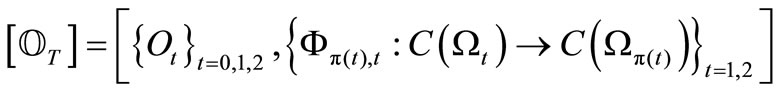
Let  be the root of a tree T. Let
be a sequential causal observable with the realization  in
in . Thus we have the statistical measurement
  , where
 . Assume that we know that the measured value
  obtained by the measurement
  belongs to
 . Then, by (4), we can infer that (S) the probability
  that y belongs to
  is given by
 (19)
(19)
Note that we can regard that  . That is, there uniquely exists
  such that
 (20)
(20)
for any observable  in
in 
 . Here, we used the following notation:
Define the observable 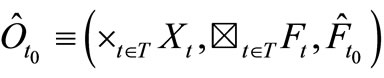 such that
Then, we can define the Bayes operator
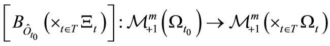 by (20).
Thus, as the generalization of Theorem 2, we have:
Theorem 3. [Causal Bayes’ theorem in classical measurements]. Let  be the root of a tree T. Let

be a sequential causal observable with the realization . Thus we have the statistical measurement
 , where
 . Assume that we know that a measured value obtained by the statistical measurement
 belongs to
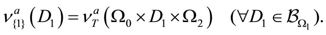
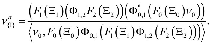
 . Then, there is a reason to infer that the mixed state
 after the statistical measurement
 is given by
 .
.
Proof. The proof is similar to the proof of Theorem 2. Thus, we omit it.
Remark 6. In Theorem 3, we see that
(T) 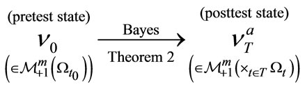
which is the generalization of the (J).
The following example promotes the understanding of Theorem 3.
Example 1. [The simple case such that ]. Consider a particular case such that
  is series ordered set, i.e.,
 . And consider a causal relation
 , that is,
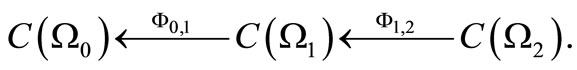
Further consider sequential causal observable
 .
.
Let 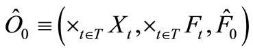 be its realization. Note, by the Formula (3), that,
Putting , we have the measurement
 (21)
(21)
Let  be the posttest state in
(T), that is,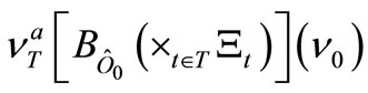 . Define
 such that
Then, we see that
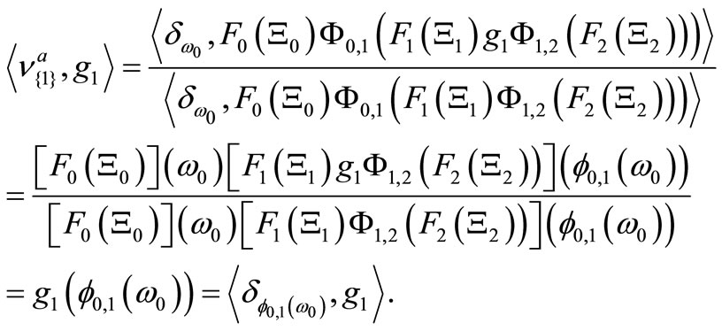
That is because we see that, for any observable  in
in ,
,
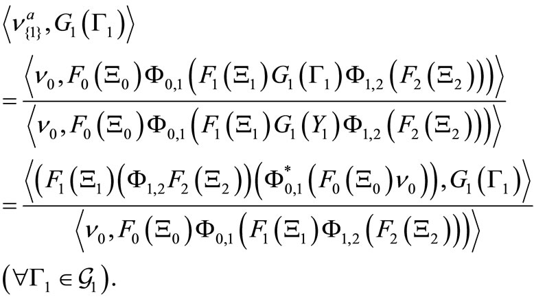 (22)
(22)
Example 2. [Continued from the above example]. For each , assume that
  is deterministic, that is, there exists a continuous map
  satisfying (12). And, putting
 , consider the measurement
 .
.
Then, we see, by (22), that, for any  in
in ,
,
Thus, we see that
 (23)
(23)
Further we easily see that
4.2. Causal Fisher-Bayes Method in Classical 
Now we can present Corollary 2 (i.e., regression analysis in a wide sense) as follows.
(U) 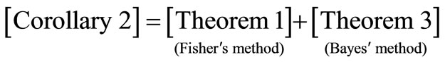
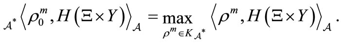
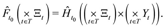
Corollary 2. [Causal Fisher-Bayes method (i.e., Regression analysis in a wide sense)]. Let  be the root of a tree T. Let
be a sequential causal observable with the realization  Assume the statistical measurement
 . And assume that we know that a measured value obtained by the measurement
  belongs to
 . Then, there is a reason to infer that the mixed state
  after the measurement
 is given by
 . Here, the
  is defined by
 (24)
(24)
Remark 7. Note that Fisher maximum likelihood method and Bayes’ theorem are hidden in Corollary 2. That is, Corollary 2 includes the following procedure:
(V) 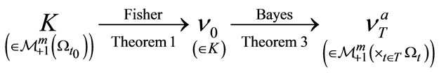
which is the generalization of the (L).
Answer 1. [Answer to Problem 1 (Q)]. Now we can answer Problem 1 (Q) as follows. The (17) says that
 . Thus, using (23), we see that
 . Also, note that (17) and (23) are consequences of Corollary 2. Hence, the calculation (18) is justified by Corollary 2.
Remark 8. As mentioned in Section 1, in our research [2-8], we have been concerned with the problem (A). Particularly, in [6], we discussed Corollary 2 in the commutative  -algebra
 . However, this was somewhat shallow, since “max” is not proper in
  but
but . Now we believe that fundamental statements concerning statistics should be always asserted in the framework of
 . Also, note that Corollary 2 is the natural generalization of Theorem 6.3 in [5].
5. Conclusions
In this paper, we devote ourselves to the problem (A) in the light of the quantum mechanical word view (cf. [7,8]). And, we show that regression analysis, which is the most fundamental in statistics, is formulated as Corollary 2 in SMT (i.e., statistical measurement theory). We believe that Corollary 2 is the finest formulation of regression analysis, since no clear formulation can be presented without the answer to the problem (A). Also, note that Corollary 2 (or, the (U)) implies that even the conventional classification of (Fisher’s) statistics and Bayesian statistics should be reconsidered.
We expect that there is a great possibility that our proposal (i.e., statistics is based on statistical measurement theory) will be generally accepted. We of course know that the conventional statistics methodology can be good applied in many fields. Hence, we hope that our methodology in the light of the quantum mechenical word view should be examined from various points of view.
REFERENCES
- A. Kolmogorov, “Foundations of the Theory of Probability (Translation),” 2nd Edition, Chelsea Pub Co., New York, 1960,
- S. Ishikawa, “Fuzzy Inferences by Algebraic Method,” Fuzzy Sets and Systems, Vol. 87, No. 2, 1997, pp. 181- 200. doi:10.1016/S0165-0114(96)00035-8
- S. Ishikawa, “A Quantum Mechanical Approach to Fuzzy Theory,” Fuzzy Sets and Systems, Vol. 90, No. 3, 1997, pp. 277-306. doi:10.1016/S0165-0114(96)00114-5
- S. Ishikawa, “Statistics in Measurements,” Fuzzy Sets and Systems, Vol. 116, No. 2, 2000, pp. 141-154. doi:10.1016/S0165-0114(98)00280-2
- S. Ishikawa, “Mathematical Foundations of Measurement Theory,” Keio University Press Inc., Tokyo, 2006, pp. 1-335. http://www.keio-up.co.jp/kup/mfomt/
- S. Ishikawa, “Fisher’s Method, Bayes’ Method and Kalman Filter in Measurement Theory,” Far East Journal of Theoretical Statistics, Vol. 29, No. 1, 2009, pp. 9-23.
- S. Ishikawa, “A New Interpretation of Quantum Mechanics,” Journal of Quantum Information Science, Vol. 1, No. 2, 2011, pp. 35-42. doi:10.4236/jqis.2011.12005
- S. Ishikawa, “Quantum Mechanics and the Philosophy of Language: Reconsideration of Traditional Philosophies,” Journal of Quantum Information Science, Vol. 2, No. 1, 2012, pp. 2-9.
- G. J. Murphy, “C*-Algebras and Operator Theory,” Academic Press, London, 1990.
- J. von Neumann, “Mathematical Foundations of Quantum Mechanics,” Springer Verlag, Berlin, 1932.
- K. Yosida, “Functional Analysis,” 6th Edition, SpringerVerlag, Berlin, 1980.
- E. B. Davies, “Quantum Theory of Open Systems,” Academic Press, London, 1976.
Appendix
As mentioned in Section 3.1, we have to prove the following theorem.
Theorem 4. [Existence theorem of product observable]. Let  and
and  be observables in a
  -algebra
 . Then, there exists the product observable
  in
in .
.
Proof. Let  [resp.
 ;
; ] be the smallest
  -field including
  [resp.
 ;
; ]. That is, for each
 , consider
 such that
and
Note, by the Hopf extension theorem (cf. Remark 1), that it suffices to show that, for any , it holds:
which is equivalent to the following equality. That is, for any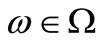 , it holds:
 (25)
(25)
However, it is easily seen since  and
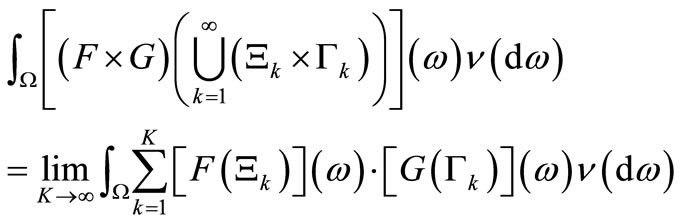
and  can be regarded as probability spaces. And therefore, we have the product probability space
 . This imlies that the equality (25) holds. This completes the proof.
Remark 9. The above proof is applicable to the realization of a sequential causal observable  in the case of an infinite T under a similar condition such that the Kolmogorov extension theorem holds (cf. [1]). Also, in quantum case (i.e.,
 ), it is well known that the weak convergence (1) in
  can be identified with the weak convergence in
 , therefore, we see, by a usual way (cf. [10,11]), that Theorem 4 holds under the commutativity condition (2).