Energy and Power Engineering
Vol. 4 No. 6 (2012) , Article ID: 25085 , 17 pages DOI:10.4236/epe.2012.46064
Fault Classification and Localization in Power Systems Using Fault Signatures and Principal Components Analysis
1Electrical Engineering Department, Tafila Technical University, Tafila, Jordan
2Department of Electrical and Computer Engineering, Western Michigan University, Kalamazoo, USA
3Energy Engineering Department, German Jordanian University, Amman, Jordan
4School of Natural Resources Engineering, Jordan University of Science and Technology, Amman, Jordan
Email: qsafasfeh@ttu.edu.jo, abdelqader@wmich.edu
Received May 4, 2012; revised June 20, 2012; accepted July 5, 2012
Keywords: Fault Detection and Classification; Protective Relaying; PCA; PSCAD
ABSTRACT
A vital attribute of electrical power network is the continuity of service with a high level of reliability. This motivated many researchers to investigate power systems in an effort to improve reliability by focusing on fault detection, classification and localization. In this paper, a new protective relaying framework to detect, classify and localize faults in an electrical power transmission system is presented. This work will extract phase current values during ( )th of a cycle to generate unique signatures. By utilizing principal component analysis (PCA) methods, this system will identify and classify any fault instantaneously. Also, by using the curve fitting polynomial technique with our index pattern obtained from the unique fault signature, the location of the fault can be determined with a significant accuracy.
1. Introduction
Fault detection and localization is a focal point in the research of power systems area since the establishment of electricity transmission and distribution systems. The objectives of a power system fault analysis is to provide enough information to understand the reasons that lead to an interruption and to, as soon as possible, restore the handover of power, and perhaps minimize future occurrences if possible at all. Analysis should indeed provide us with an understanding of the network that can lead to producing a set of preventive measures which can be implemented to reduce the likelihood of equipment damage. Circuit breakers and other control elements are designed to help protective relays to take appropriate actions [1,2] and thus minimize damage and length of interruption. Prompt detection of a fault will have a significant impact on the equipment safety since it will engage the circuit breakers instantaneously and before any significant damage occurs. In recent years, with an increase in the number of power system networks within one control center, the behavior and effect of faults became more complex and as a result, fault impacted area has expanded. Researchers in applied mathematics and signal processing have developed many techniques for the detection, classification and localization of faults in electrical power systems and used them in conjunction with relaying and protection devices. Recent tools include Artificial Neural Network (ANN) and Wavelets among other powerful pattern recognition and classification tools. ANN based algorithms depend on indentifying the different patterns of system variables using impedance information. The proposed neural network architectures suffer from a large number of training cycles and a high computational burden. Another significant drawback for using ANN is that the resolution is not efficient since it can be a very sparse network with the need for large size training data adding an additional burden on its computational complexity [3-6]. Wavelet transform has been proposed by many to decompose voltage and current waves in an effort to identify a fault. It has been reported that wavelet transform based methods for fault detection are fast and effective analysis methods [7]. Others incorporated wavelet transform with other methods such as Probabilistic Neural Network (PNN), adaptive resonance theory, adaptive neural fuzzy inference system, and support vector machines [8-11]. Fuzzy logic was also combined with discrete Fourier transform, adaptive resonance theory, principles of estimation and independent component analysis to enhance performance [11-16]. In comparison with ANN, Fuzzy logic systems are subjective and heuristic and in general, they are simpler than the wavelet transform or the neural network based techniques. Unfortunately, most of the available tools for fault detection and classification are not efficient and are not investigated for real time implementation [4]. There is a need for new algorithms that have high efficiency, general applicability, and suitable for real time usage. In this work, we present a protection scheme consisting of three stages; the first stage includes the fault detection and classification based on patterns generated from phase current while the second stage is to initiate the classification process via PCA to declare the occurrence of a fault, if any, and its type. For the third stage, and once a fault is declared, a localization process is initiated to determine the fault location by combining our pattern indices generated from the unique fault signatures and the polynomial curve fitting technique. This framework is illustrated in Figure 1.
2. Signature Estimation of Fault Signal
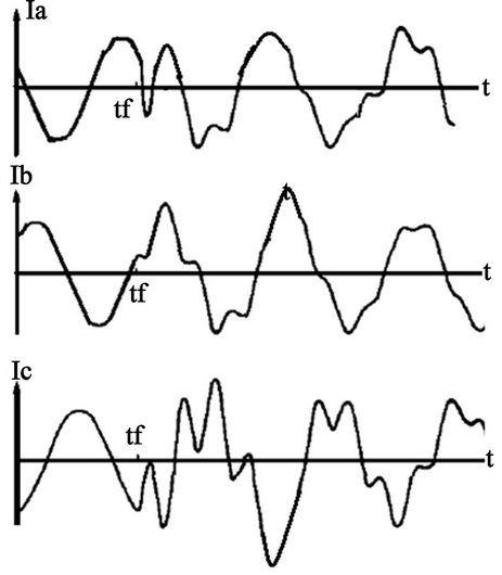
Figure 2 represents a 3-phase system signals in the time domain extracted from a power system. In Part a, the three current signals from each phase are shown while part b is showing the diagram of the difference signal, DS, from an unbalanced three-phase system.
The difference signal DS between current signal and its previous reading at each ( )th of a cycle is generated at the sending end of the transmission line. The difference signal, shown in Figure 2(b), at each instant of time is assumed to model a line equation of the form:
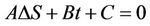 (1)
(1)
where A, B and C are constant derived from line specific intersect points. Once DS is modeled using the line equation given in Equation (1), it is used to transform the data into a phasor domain by transforming each value of the difference signal as a magnitude and phase of its line tors in the ρ-λ space as
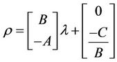 (2)
(2)
The magnitude and phase values for this new vector representation are computed using Equations (3) and (4) as follows:
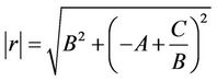 (3)
(3)
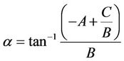 (4)
(4)
where  and
and  are the mathematical magnitude and phase at each value of the DS signal, respectively. Considering three variables for the three phases a, b, and c, we will produce the following 3-phase set of equations:
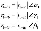 (5)
(5)
where ,
,  , and
, and  are the mathematical magnitude values at one instant of DS signal for phase a, b, and c, receptively and
 ,
,  , and
, and  are the mathematical phase values at one instant of the of DS signal for phase a, b and c, receptively. Our data transformation is followed by a transformation into symmetrical components via the symmetrical components technique [17], which allows for systematic analysis and
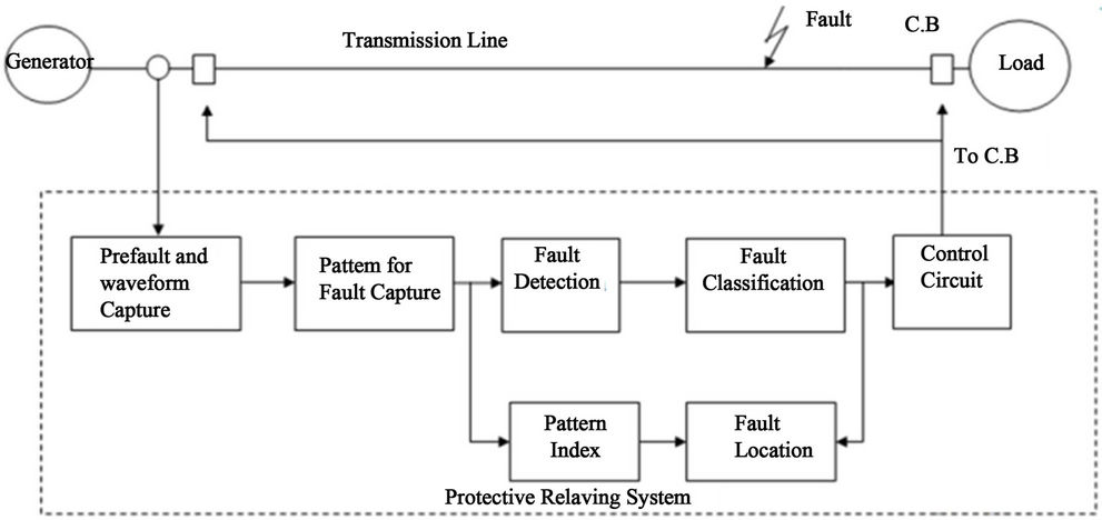
Figure 1. An illustration of the electrical protective relaying system proposed in this work showing the multistage process involved.
 (a)
(a)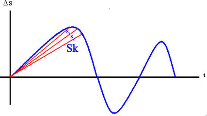 (b)
(b)
Figure 2. Unbalanced system signals: (a) each phase signal and (b) difference signal of current wave for phase a under a fault condition.
design of three phase systems as shown in Equation (6). In the left hand side of Equation (6) are the sought symmetric quantities while the right hand side is the system phasor quantities. In Equation (7) we replace the phasor quantities of Equation (6) by our transformed data of the difference signal DS,
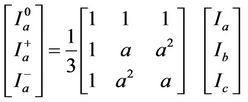 (6)
(6)
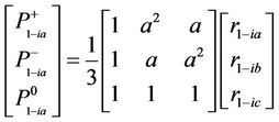 (7)
(7)
This allows us to capture the symmetric components of DS by generating positive and negative patterns of each instant. Hence for total k samples, the symmetrical components will be:
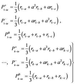 (8)
(8)
Leading to
By computing  and
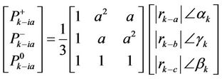
and  over a time series all within (1/4)th of a cycle, we generate, shown in Equation (9), the positive and negative signatures which is a model for any unbalanced and nondeterministic time threephase system which was allowed by symmetrical components method utilization.
 (9)
(9)
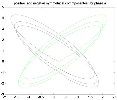
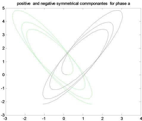
Figure 3 shows a plot of the unique signature of phase a in a 3-phase system with a fault a-g only while samples of other signatures are shown in the experimental work in Section 4.
The output of this process will then be supplied into the classification process to detect the fault and obtain a classification for the event. This proposed work is implemented and simulated using several PSCAD simulations. In Figure 4 a functional block diagram for the framework steps is shown.
3. Principal Component Analysis (PCA) Based Fault Detection and Classification Method
PCA has proven to achieve excellent results in feature extraction and data reduction in large datasets [18-20]. Typically PCA is utilized is to reduce the dimensionality of a dataset in which there is a large number of interrelated variables while the current variation in the dataset is maintained as much as possible [21]. The principal
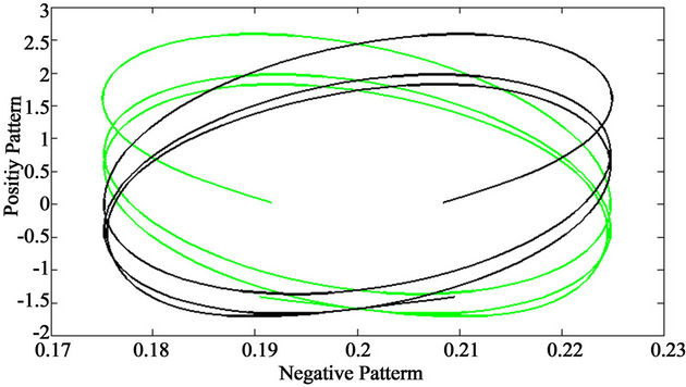
Figure 3. A plot of the unique signature of phase a in a 3-phase system with a fault a-g only.
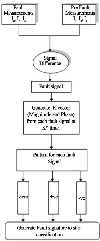
Figure 4. Detailed procedure followed to generate the signatures; difference signal is used thought data transformation and symmetrical component method to obtain a unique signature of every event.
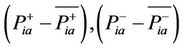
components (PCs) are calculated using the covariance matrix after a simple normalization procedure. The covariance matrix is, then calculated for these patterns simply as
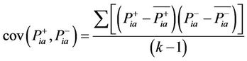 (10)
(10)
where  and
and , generated earlier per Equation (9), are the positive and negative patterns respectively,
  and
and  the mean of
 ,
,  respectively, and k is the number of samples used. Projection into the PC space is performed by using
 (11)
(11)
where C is the covariance matrix; αi is the principal component in the ith dimension and  is its corresponding eigenvalue. Projecting the normalized data
 onto the principal components, a new vector of data will be generated (PC1, PC2). Accompany the usage of PCA for feature extraction is the usage of a similarity measure usually as a distance measure. These may include Chebyshev, Euclidean, Manhattan, City Block, Canberra, and Minkowski, [22,23]. In this paper, the Euclidean distance measure is adapted as shown in Equation (12).
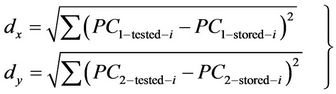 (12)
(12)
The classification process of a fault is divided into two stages; the first is the training procedure using all signatures generated prior to testing, to enforce their projections onto the principal components space. The second stage is the testing process, in which steps in Figure 3 are followed to project the test pattern onto PCA space followed by measuring for similarity of the PCs using the minimum distance between the stored projections and test one. This minimum distance will identify a match of a pattern to a fault or no fault at all. In Figure 5 we display the general framework for fault classification.
4. Experimental Results on Fault Detection and Classification
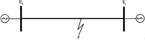
Using the simulation package PSCAD, transmission line model shown in Figure 6 is used to simulate our framework. The network is composed of two sources, 220 kv each, that are connected by the transmission line with zero sequence parameter Z(0) = 82.5 + j308 Ω and a positive sequence impedance Z(1) = 8.25 + j94.5 Ω while ES = 220 kv and ER = 220∠δ kv.
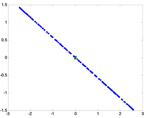
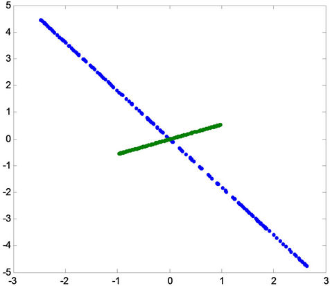
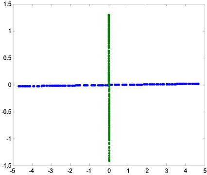
We also, to show the validity of our algorithm on a more complex network, simulate our framework using a 6 bus network as shown in Figure 6(b). For this bus, the source voltages are at 400 kv each and the transmission line parameters are the same as the previous transmission line model. Positive and negative patterns for the 3-phase system are displayed by Figures 7-10 and classification results are presented in Tables 1 and 2. The result of “No Fault” is the healthy condition event which we show its pattern in Figure 7. It is clear from Figure 7 that the signature of each event is completely unique. A viewer for the signatures can easily identify the pattern of the faulty phase and declare the type of the fault from Figures 8 and 9. Projections into PCA results are also demonstrated in Figures 10-12. The Power system fault classifier was tested to classify the faults into a-g, b-g, cg, ab-g, ac-g, bc-g, ab, ac, bc, or abc using a total 220 samples for testing.
Classification accuracy is presented in the confusion matrix in Table 1. These results were obtained with one template/pattern in the training data set. Table 2 displays the results storing two templates in the training set. The error percentage in the later case is zero. Results are considered to be of significant improvement over the traditional approaches.
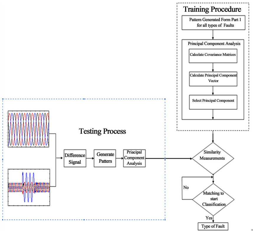
Figure 5. The general framework for fault classification using principal component analysis as a tool for feature extraction of fault signatures.
 (a)
(a)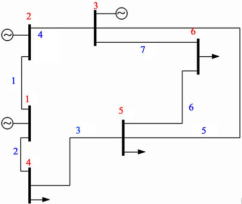 (b)
(b)
Figure 6. Using PSCAD simulation package, our framework was tested using (a) a 220 kv transmission lines and (b) a 400 kv 6-bus network.
5. Fault Localization
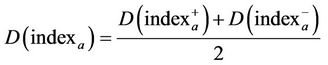
This framework can also be expanded to include a fault localization procedure. In this paper, the fault location is calculated by combining the curve fitting polynomial technique with our unique pattern indices that are generated from the signatures as follows:
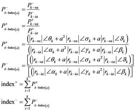 (13)
(13)
where ,
,  are the positive and negative Pattern indices for phase a. Using curve fitting, a training set is produced for the positive and negative pattern
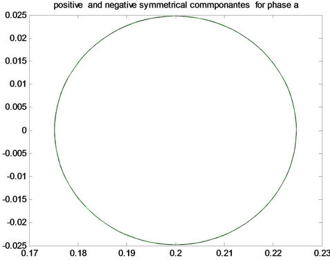 (a)
(a)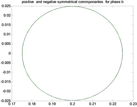 (b)
(b)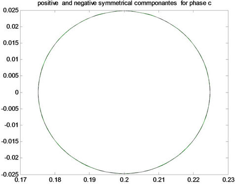 (c)
(c)
Figure 7. Positive and negative pattern for each phase (phase a, phase b and phase c) for healthy condition.
indices and their fault corresponding distances. The Positive and negative indices are calculated at different loca-
 A(a)
A(a) 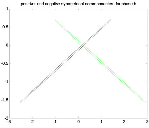 A(b)
A(b) 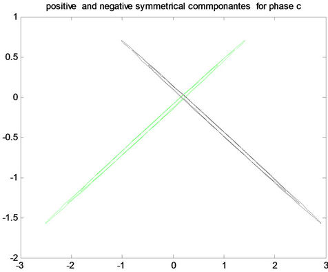 A(c)
A(c)
 B(a)
B(a) 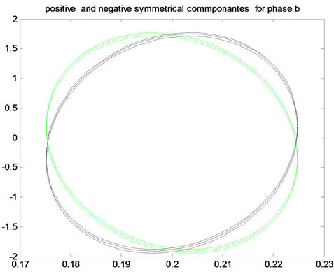 B(b)
B(b) 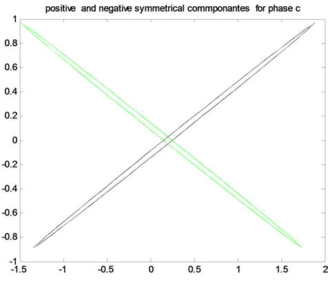 B(c)
B(c)
 C(a)
C(a) 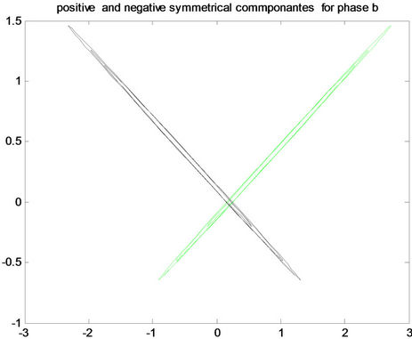 C(b)
C(b) 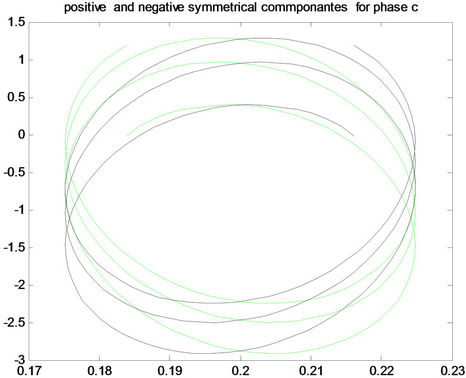 C(c)
C(c)
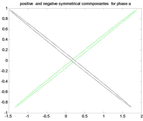
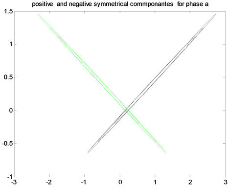
Figure 8. Positive and negative pattern for fault a-g in the first row, for fault b-g in the middle, and for fault c-g in the last row for (A) phase a, (B) phase b and (C) phase c.
 A(a)
A(a) 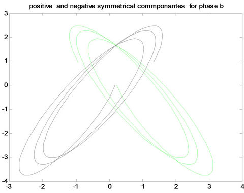 A(b)
A(b) 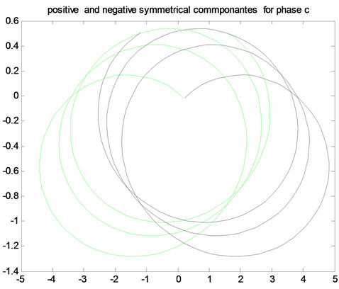 A(c)
A(c)
 B(a)
B(a) 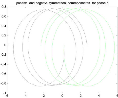 B(b)
B(b) 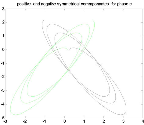 B(c)
B(c)
 C(a)
C(a) 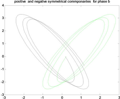 C(b)
C(b)  C(c)
C(c)
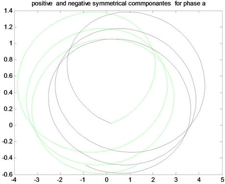
Figure 9. Positive and negative pattern for fault ab-g in the first row, for fault ac-g in the middle, and for fault bc-g in the last row for (A) phase a, (B) phase b and (C) phase c.
 (a)
(a)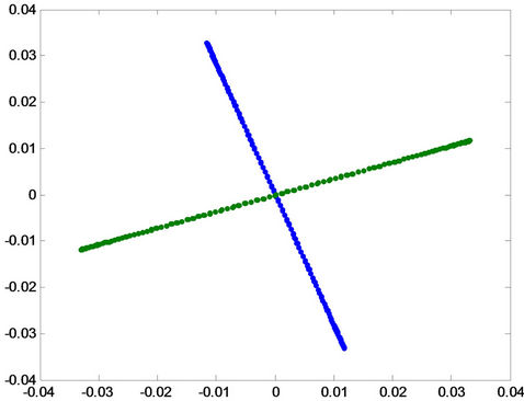 (b)
(b)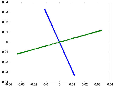 (c)
(c)
Figure 10. Projection of the patterns onto principal component for healthy condition.
tions (5, 25, 35, 50, 75, 95) km from sending end of the transmission line with a variety of operating conditions such as power angles and source impedance but at a spe-
 A(a)
A(a) 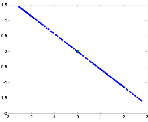 A(b)
A(b) 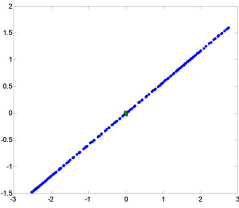 A(c)
A(c)
 B(a)
B(a) 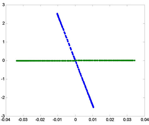 B(b)
B(b) 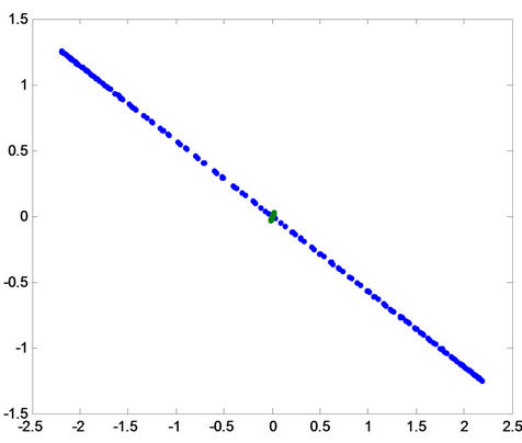 B(c)
B(c)
 C(a)
C(a) 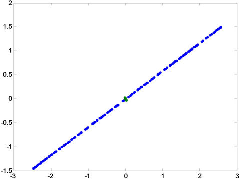 C(b)
C(b)  C(c)
C(c)
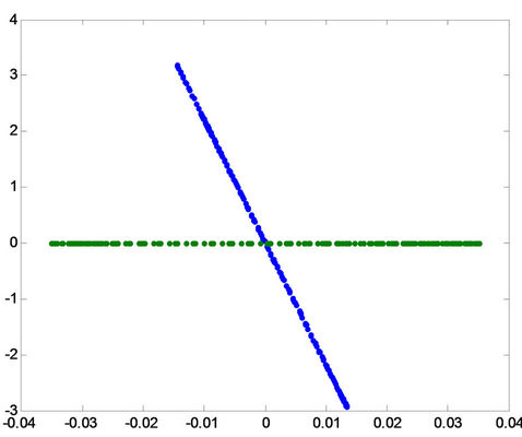
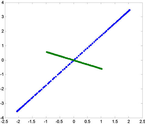
Figure 11. Projection of the patterns onto principal compo-nent for fault a-g in the first row, for fault b-g in the middle, and for fault c-g in the last row for (A) phase a, (B) phase b and (C) phase c.
 A(a)
A(a) 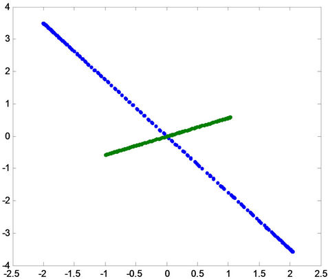 A(b)
A(b) 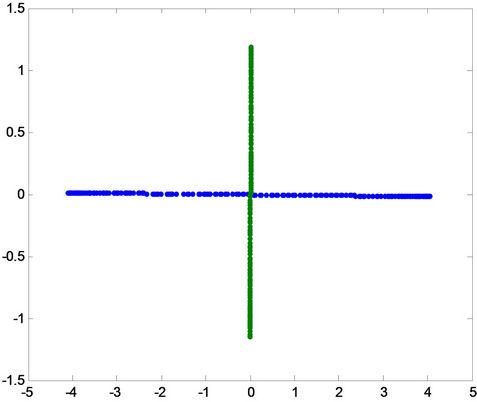 A(c)
A(c)
 B(a)
B(a) 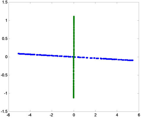 B(b)
B(b) 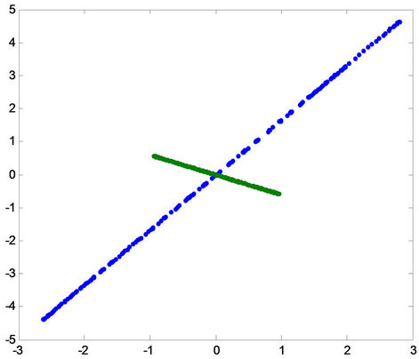 B(c)
B(c)
 C(a)
C(a) 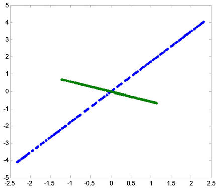 C(b)
C(b) 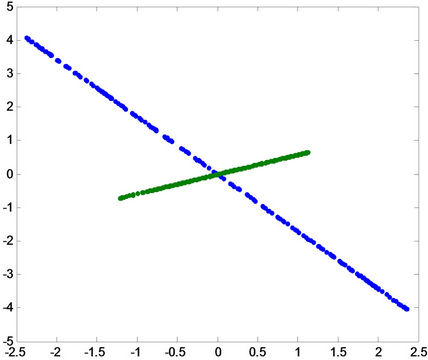 C(c)
C(c)
Figure 12. Projection of the patterns onto principal component for fault ab-g in the first row, for fault ac-g in the middle, and for fault bc-g in the last row for (A) phase a, (B) phase B and (C) phase c.
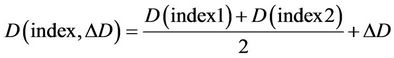
cific fault resistance. To estimate the fault location, the positive and negative Pattern indices of the real incident/test signals are determined and projected onto the fitted curve polynomial. An average of the two readings is taken as the fault location.
 (14)
(14)
where  is the average distance of the previous estimates taken to be an accurate estimate of the fault location. The estimated distance in the first polynomial curve fitting is dependent on the specific value of the fault resistance and so if the fault to occur at a different values of fault resistance, that is, at a fault resistance not used in the first polynomial curve fitting, then an error in the distance estimate will occur. However, the error can be compensated by accounting for the difference in the fault resistance. That is, ∆R, the difference between the new fault resistance and the one used in the training, is used to generate a new polynomial curve to extract the corresponding ∆D. Upon testing and if there is any change in fault resistance then ∆D, the error in the distance, will be added to the calculated fault distance as shown in (15).
 (15)
(15)
The error in fault location is given as (16).
 (16)
(16)
where D is the estimated fault distance,  is the exact fault distance, and L is the transmission line total length, the functional block diagram as shown in Figure 13.
6. Experimental Results on Fault Localization
Using the simulation package PSCAD, transmission line model shown in Figure 6(a) is used to simulate our framework. The network is composed of two sources, 220 kv each, that are connected by the transmission line with zero sequence parameter Z(0) = 82.5 + j308 Ω and a positive sequence impedance Z(1) = 8.25 + j94.5 Ω while ES = 220 kv and ER = 220∠δ kv.
We also, to show the validity of our algorithm on a more complex network, simulate our framework using a 6-bus network as shown in Figure 6(b). For this bus, the source voltages are at 400 kv each and the transmission line parameters are the same as the previous transmission line model. After applying the fault classification was presented in our paper Fault Classification of Power Systems Using Fault Signatures and Principal Components Analysis Table 3 provides the fault location estimates for a-g, ab-g, and ab faults at various network con-
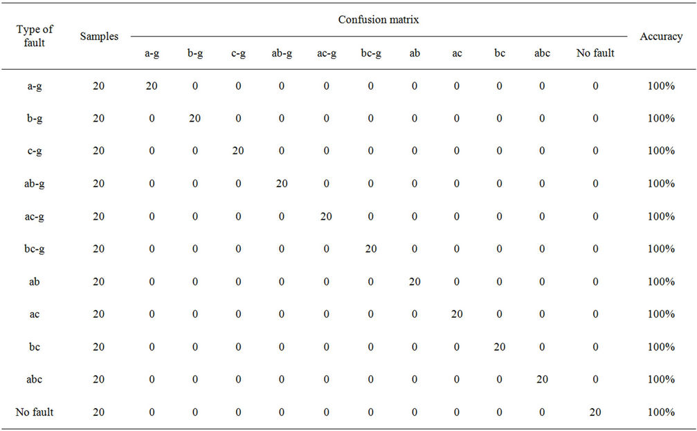
Table 1. Classification performance using one template for each fault type in the training set producing a 94.54% average accuracy.
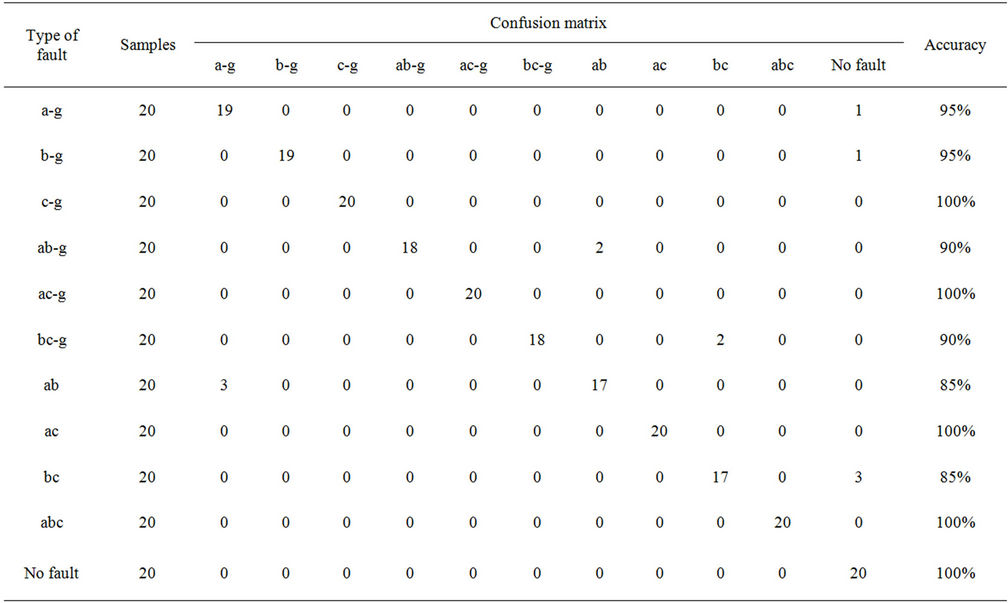
Table 2. Classification performance by using two templates for each fault type in the training set producing 100% accuracy.
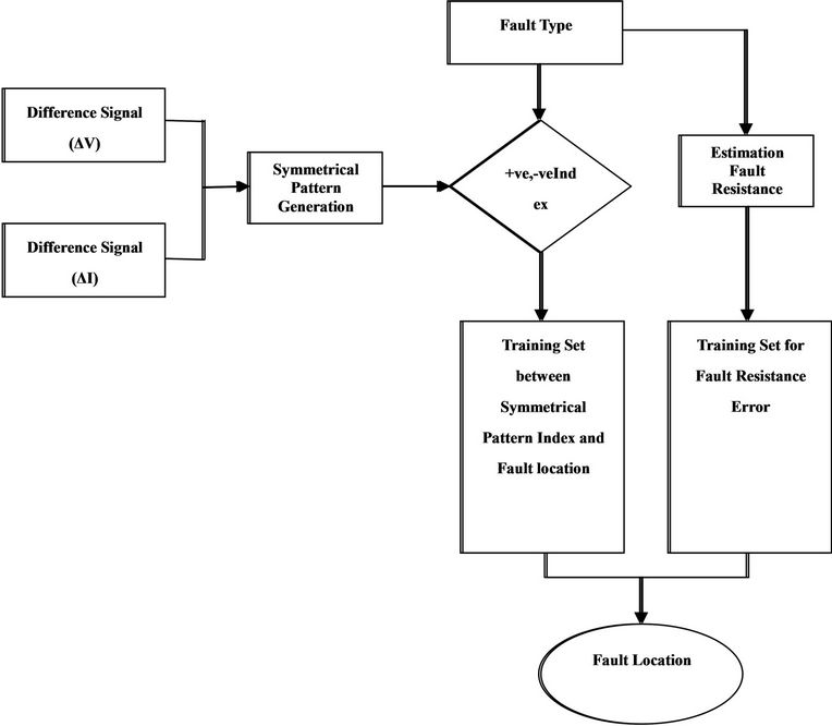
Figure 13. Functional block diagram for fault location based on patterns indices.
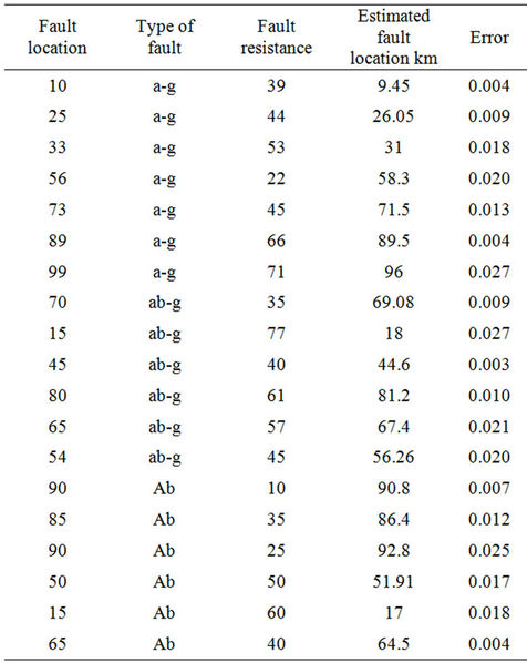
Table 3. Fault location for different fault.
ditions. Maximum error is 2.7% in ab-g fault at 15 km from relaying point with fault resistance of 77 Ω and minimum error of 0.3% in ab-g at a 45 km from relaying point with fault resistance of 40 Ω. Table 4 shows the results for fault detection, classification and fault location for a 6 bus network with maximum error of 3% in cases of bc-g and ab faults with a 5 Ω and a 100 Ω fault resistance respectively. A functional block diagram for fault location based on patterns indices is shown in Figure 2.
7. Conclusions
This paper presented a new electrical protective relaying system framework to detect, classify, and localize any fault type in electrical power system using pattern recognition. The detection and classification process depends on unique signatures generated from the difference between preand post-fault current signal values during a ( )th of a cycle only. Fault signatures were projected into the PC space and stored, as a training set, for system monitoring. This protective relaying framework is of a general applicability such that it can be deployed at one end of a transmission line without the need for communication devices between the two ends. The Power system fault classifier was tested to classify all fault types
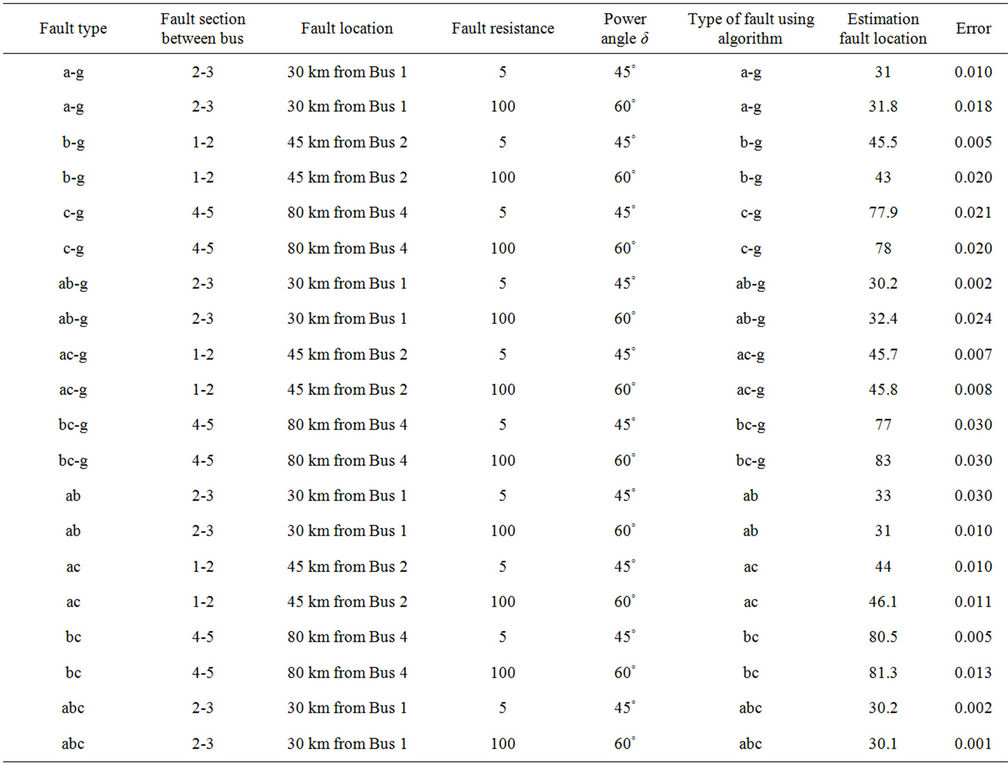
Table 4. Fault detection, classification and localization for a 6-bus network.
into a-g, b-g, cg, ab-g, ac-g, bc-g, ab, ac, bc, and abc with a total of 220 fault samples for algorithm simulation and testing. The classification accuracy was calculated to be at 94.54% using only one template per fault signature in the training set, and was improved to 100% by increasing the templates per fault signature to two. Determining fault location was also considered by combining polynomial curve fitting technique with the pattern index ratio of both the voltage signal and current signal unique signatures. The error in fault location is found to be below 2.7%. This proposed work is computationally simple, efficient, and can be used in real-time applications. This work can be easily expanded to more complex networks and can be used in distribution systems.
REFERENCES
- M. Kezunovic, et al., “Automated Fault Analysis Using Neural Network,” 9th Annual Conference for Fault and Disturbance Analysis, Texas A&M University, College Station, Texas, March 1994.
- M. Kezunovic and I. Rikalo, “Detect and Classify Faults Using Neural Nets,” IEEE Computer Applications in Power, Vol. 9, No. 4, 1996, pp. 42-47. doi:10.1109/67.539846
- K. Ferreira, “Fault Location for Power Transmission Systems Using Magnetic Field Sensing Coils,” Master Thesis, Worcester Polytechnic Institute, Worcester, April 2007.
- A. Jain, A. Thoke and R. Patel, “Fault Classification of Double Circuit Transmission Line Using Artificial Neural Network,” International Journal of Electrical and Electronics Engineering, Vol. 1, No. 4, 2008, pp. 230-235.
- A. Jain and A. Thoke, “Classification of Single Line to Ground Faults on Double Circuit Transmission Line Using ANN,” International Journal of Computer and Electrical Engineering, Vol. 1, No. 2, 2009, pp. 196-203.
- M. Sanaye-Pasand and H. Khorashadi-Zadeh, “Transmission Line Fault Detection & Phase Selection Using ANN,” International Conference on Power Systems Transients— IPST, New Orleans, 2003, pp. 1-6.
- H. Zheng-You, C. Xiao-Qing and F. Ling, “Wavelet Entropy Measure Definition and Its Application for Transmission Line Fault Detection and Identification (Part II: Fault Detection in Transmission Line),” International Conference on Power System Technology, Chongqing, 22-26 October 2006, pp. 1-5.
- K. S. Swarup, N. Kamaraj and R. Rajeswari, “Fault Diagnosis of Parallel Transmission Lines Using Wavelet Based ANFIS,” International Journal of Electrical and Power Engineering, Vol. 1, No. 4, 2007, pp. 410-415.
- V. Malathi and N. Marimuthu, “Multi-Class Support Vector Machine Approach for Fault Classification in Power Transmission Line,” IEEE International Conference on Sustainable Energy Technologies ICSET 2008, Singapore, 24-27 November 2008, pp. 67-71.
- S. El Safty and A. El-Zonkoly, “Applying Wavelet Entropy Principle in Fault Classification, International,” Journal of Electrical Power & Energy Systems, Vol. 31, No. 10, 2009, pp. 604-607. doi:10.1016/j.ijepes.2009.06.003
- J. Upendar, C. P. Gupta and G. K. Singh, “Discrete Wavelet Transform and Genetic Algorithm Based Fault Classification of Transmission Systems, National Power Systems Conference (NPSC-2008),” Indian Institute of Technology, Bombay, December 2008, pp. 223-228.
- D. Biswarup and V. Reddy, “Fuzzy-Logic-Based Fault Classification Scheme for Digital Distance Protection,” IEEE Transactions on Power Delivery, Vol. 20, No. 1, 2005, pp. 609-616.
- K. Razi, M. Hagh and G. Ahrabian, “High Accurate Fault Classification of Power Transmission Lines Using Fuzzy Logic,” International Power Engineering Conference IPEC, Singapore, 3-6 December 2007, pp. 42-46.
- S. Vaslilc and M. kezunovic, “Fuzzy ART Neural Network Algorithm for Classifying the Power System Faults,” IEEE Transactions on Power Delivery, Vol. 20, No. 2, 2005, pp. 1306-1314. doi:10.1109/TPWRD.2004.834676
- S. Samantaray, P. Dash and G. Panda, “Transmission Line Fault Detection Using Time-Frequency Analysis,” IEEE Indicon 2005 Conference, Chennai, 2005, pp. 162-166.
- E. Styvaktakis, M. Bollen and I. Gu, “Automatic Classification of Power System Events Using rms Voltage Measurements,” IEEE Power Engineering Society Summer Meeting, Chicago, 25 July 2002, pp. 824-829.
- H. Saadat, “Power System Analysis,” McGraw Hill, New Yoek, 2002.
- I. Jollife, “Principal Component Analysis,” Verlag, Springer, 1986.
- J. Karhunen and J. Joutsensalo, “Generalizations of Principal Component Analysis, Optimization Problems, and Neural Networks,” Neural Networks, Vol. 8, No. 4, 1995, pp. 549-562. doi:10.1016/0893-6080(94)00098-7
- S. Nayar and T. Poggio, “Early Visual Learning,” Oxford University Press, New York, 1996.
- I. Abdel-Qader, S. Pashaie-Rad, O. Abudayyeh and S. Yehia, “PCA-Based Algorithm for Unsupervised Bridge Crack Detection,” Advances in Engineering Software, Vol. 37, No. 12, 2006, pp. 771-778. doi:10.1016/j.advengsoft.2006.06.002
- D. Widdows, “Geometry and Meaning,” University of Chicago Press, Chicago, 2003.
- Q. Alsafasfeh, I. Abdel-Qader and A. Harb, “Symmetrical Pattern and PCA Based Framework for Fault Detection and Classification in Power System,” Proceedings of IEEE Electro/Information Technology Conference, Normal, 24 May 2010, pp. 1-5.