Journal of Signal and Information Processing
Vol. 4 No. 2 (2013) , Article ID: 31061 , 13 pages DOI:10.4236/jsip.2013.42025
A Modal Identification Algorithm Combining Blind Source Separation and State Space Realization
![]()
Stress Engineering Services, Inc., Houston, USA.
Email: scot.mcneill@stress.com
Copyright © 2013 Scot McNeill. This is an open access article distributed under the Creative Commons Attribution License, which permits unrestricted use, distribution, and reproduction in any medium, provided the original work is properly cited.
Received January 23rd, 2013; revised February 28th, 2013; accepted March 9th, 2013
Keywords: Modal Identification; Blind Source Separation; State Space Realization; Analytic Signal; Complex Modes
ABSTRACT
A modal identification algorithm is developed, combining techniques from Second Order Blind Source Separation (SOBSS) and State Space Realization (SSR) theory. In this hybrid algorithm, a set of correlation matrices is generated using time-shifted, analytic data and assembled into several Hankel matrices. Dissimilar left and right matrices are found, which diagonalize the set of nonhermetian Hankel matrices. The complex-valued modal matrix is obtained from this decomposition. The modal responses, modal auto-correlation functions and discrete-time plant matrix (in state space modal form) are subsequently identified. System eigenvalues are computed from the plant matrix to obtain the natural frequencies and modal fractions of critical damping. Joint Approximate Diagonalization (JAD) of the Hankel matrices enables the under determined (more modes than sensors) problem to be effectively treated without restrictions on the number of sensors required. Because the analytic signal is used, the redundant complex conjugate pairs are eliminated, reducing the system order (number of modes) to be identified half. This enables smaller Hankel matrix sizes and reduced computational effort. The modal auto-correlation functions provide an expedient means of screening out spurious computational modes or modes corresponding to noise sources, eliminating the need for a consistency diagram. In addition, the reduction in the number of modes enables the modal responses to be identified when there are at least as many sensors as independent (not including conjugate pairs) modes. A further benefit of the algorithm is that identification of dissimilar left and right diagonalizers preclude the need for windowing of the analytic data. The effectiveness of the new modal identification method is demonstrated using vibration data from a 6 DOF simulation, 4-story building simulation and the Heritage court tower building.
1. Introduction
An introduction to blind source separation applied to modal identification is provided in this section, along with a review of previous developments in the literature.
1.1. Blind Source Separation Applied to Modal Identification
In the last several years research has evolved the application of Blind Source Separation (BSS) techniques to solve the Modal ID entification (MID) problem. BSS attempts to find source components,  , with prescribed properties embedded in measured data
  . The techniques applicable for modal identification assume that the measured data is a linear mixture (as opposed to convolutive) of the components.
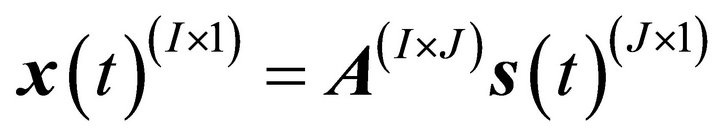
Suppose that there are I channels of measured data and J components. The relation between the components and the measured data can be written as
 (1)
(1)
where A is the (constant) mixing matrix and the dimensions have been placed parenthetically in the superscript. Note that all quantities are generally complex-valued. The objective of BSS is to simultaneously estimate the mixing matrix, A, and the vector of components, ![]() , from the observed data,
, from the observed data, . Due to the number of variables involved, this task requires a characterization of the source components,
![]() . Many BSS techniques use second order statistical information (e.g. correlation structure) to describe the components. It is appropriate to consider the inverse relationship of (1),
. Many BSS techniques use second order statistical information (e.g. correlation structure) to describe the components. It is appropriate to consider the inverse relationship of (1),
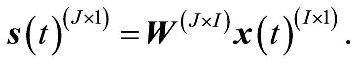 (2)
(2)
The de-mixing matrix, W, is the (generalized, if necessary) inverse of the mixing matrix, A. The BSS task is to estimate A and![]() . Assume that the rank of A is given by
. Assume that the rank of A is given by . This can easily be satisfied by judicious choice of sensor locations. If
 , then (1) is a fully determined problem for the sources,
![]() . If
. If , then (1) is an over determined problem. Similarly, if
 , then (1) is an under determined problem. Most BSS algorithms only treat the fully determined or over determined cases.
The potential application of BSS on vibration data is fairly obvious. In linear vibration, the physical responses,  , are constructed from the modal responses,
  , by multiplication of the modal matrix,
 ,
,
 (3)
(3)
One might consider using BSS to estimate both the (inverse) modal matrix and the modal responses,
 (4)
(4)
The connection with Equations (1) and (2) is immediate. The decomposition, once achieved, allows for estimation of natural frequency and damping ratios using simple SDOF methods applied to . Note that the modal matrix and modal responses are real valued if the topology of the damping matrix is restricted (e.g. proportional damping) and are otherwise complex-valued.
1.2. Discussion of Previous Developments
Early attempts at using BSS for MID are simply applied BSS methods, such as the Algorithm for Multiple Unknown Signal Extraction (AMUSE) [1] and Second Order Blind Identification (SOBI) [2] algorithms, directly to measured vibration data [3-5]. However, little insight was provided regarding the relationship between the source components identified by such algorithms to modal responses. In addition, the methods suggested were not capable of identifying complex-valued modes. This presents a problem for application to measured data as most physical structures and machinery exhibit complexvalued modes.
Recently, a framework for Blind Modal Identification (BMID) was developed to perform MID using BSS methods [6-9]. It was first shown that the SOBI algorithm is suitable for the modal identification task for systems with real-valued modes (diagonally damped systems). The SOBI algorithm finds source components in measured physical response data that are uncorrelated irrespective of time shifts relative to one another.
Specifically, the SOBI algorithm finds components that approximately produce diagonal time shifted correlation matrices. A complex-valued version of SOBI is now discussed, though the algorithm was originally presented for the real-valued mixing model. Consider the time shifted correlation matrix of observed data ,
,
 . (5)
. (5)
Here τ is a time shift, ![]() , represents the Hermetian (complex conjugate) transpose and
, represents the Hermetian (complex conjugate) transpose and  has been centralized by removing the mean from each channel. SOBI employs Joint Approximate Diagonalization (JAD) to find the demixing matrix,
  , that approximately diagonalizes several time shifted correlation matrices with time shift
 ,
,
 (6)
(6)
This problem can be solved by minimizing the off diagonal terms of  for the K correlation matrices,
 (7)
(7)
Joint approximate diagonalization was first solved in two steps: 1) prewhitening the data by transforming with a unitary matrix found from Principal Component Analysis (PCA); 2) applying the final rotation matrix obtained by applying Givens rotations on the data correlation matrix [10]. The mixing matrix was then constructed as the product of two unitary matrices. Several single-step algorithms were later developed (e.g., [11,12] and the references therein).
By appealing to the correlation structure of the modal responses,  , the source components,
 ![]() , where shown to correspond to the modal responses and the mixing matrix,
, where shown to correspond to the modal responses and the mixing matrix,  , was shown to correspond to the system mode shapes,
 . Namely, the modal responses were stated to have nearly diagonal time-shifted correlation matrices. Damping and finite data length was shown to result in nonzero off-diagonals, causing the correspondence between
  and
and ![]() to be approximate, resulting in error in the mode shapes and modal responses. This error was mitigated by introducing a windowing technique. A Gaussian window is applied to the data set before applying SOBI. Windowing the data causes the windowed modal responses to have diagonal correlation matrices, improving the quality of the estimated mixing matrix [6,7].
to be approximate, resulting in error in the mode shapes and modal responses. This error was mitigated by introducing a windowing technique. A Gaussian window is applied to the data set before applying SOBI. Windowing the data causes the windowed modal responses to have diagonal correlation matrices, improving the quality of the estimated mixing matrix [6,7].
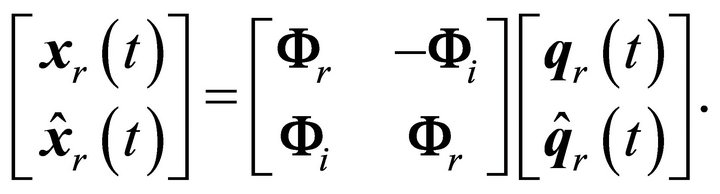
A further objective of BMID is to extend SOBI to systems with complex-valued modes (non-diagonally damped systems), allowing for estimation of complex-valued mode shapes, natural frequencies and modal damping. The complex-valued mode shapes can be expressed as,
 , (8)
, (8)
where i is the imaginary unit, and the subscripts r and i indicate the real and imaginary parts, respectively. This was accomplished simply by applying SOBI on an expanded data set. The measured data set is augmented with its Hilbert transform to yield the double-sized mixing problem,
 (9)
(9)
In (9) the  symbol indicates the Hilbert transform. Note that though Equation (9) contains the imaginary part of the complex modes, the imaginary unit is not present. Therefore all the terms are real-valued and (9) may be solved using a real-valued implementation of SOBI.
Consider the analytic signals associated with the measured data and the modal responses,
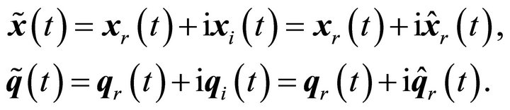 (10)
(10)
In [9] it was shown that the complex mixing problem,
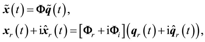 (11)
(11)
is equivalent to the double-sized problem (9). It was also noted that solving (11) instead of (9) using a complexvalued implementation of SOBI avoids a post-processing step, known as the pairing routine, needed to match the modal responses to their Hilbert transform pairs. In addition, it was suggested in reference [9] that a single-step JAD routine can be used to solve (11), and thus avoid the whitening step common in many of the early JAD algorithms. A complex-valued version of the high-performance Weighted Exhaustive Diagonalization with Gauss itErations (WEDGE) algorithm [11-13], was used to solve for the complex mode shapes and modal responses.
Many of the obstacles involved in applying BSS for MID were overcome by the proposed BMID framework. However one of the remaining limitations of the method is that the under determined case, where the number of sensors is less than the number of modes present in the measured data , cannot be solved. In practice, this issue is often addressed by band-pass filtering the measured data into two or more bandwidths where
  and applying BMID on each of the bands, separately. It is desirable from a time and effort standpoint to minimize the amount of bands necessary. In addition allowance for identification of more sources (modal responses) than sensors can allow for better quality modal parameters, as more noise modes can be identified and separated from the structural modes.
Most of the methods thus far proposed to extend BSS to the underdetermined case exploited a technique from multilinear algebra, known as Parallel Factor analysis (PARAFAC) [14-16]. The PARAFAC algorithm employed in these methods was that of [17], due to its convergence properties. In [14,15], PARAFAC was applied to the measured data directly for estimation of real and complex modes, respectively. The Blind Modal Identification for under determined data (BMIDUD) algorithm was developed by the author [16]. The algorithm applies PARAFAC to the analytic data set, composed of the measured data and corresponding Hilbert transform. After applying BMIDUD to two sets of simulated data, performance of the BMIDUD algorithm was observed to be fairly good in the underdetermined case. However, two shortcomings can be noted. First, the number of modes identified is limited by,
 (12)
(12)
The maximum number of uniquely identifiable sources for several values of I is listed in according to Table 1. Second, some residual mixing was evident in the modal auto-correlation functions. The first issue can be quite restrictive when the number of sensors is small. The second issue may result in error in modal parameter estimates.
Another approach to the underdetermined case is to assemble a large Hankel matrix from the data correlation matrices, as first suggested in [18]. This method does not suffer from the identifiability condition of Equation (12). In addition, the modal auto-correlation functions are easily obtained in a post-processing step. The method was extended in [19], where methods from state-space realization were combined with SOBI for improved modal identification. It was also shown that when dissimilar left and right diagonalizers are applied to the Hankel matrix, the correct mode shapes can be obtained without the need for windowing the data. In a related result, it was proven that the off diagonals of the modal response correlation are nonzero unless the system is conservative (i.e., does not have damping), as surmised in [6,7].
In the remainder of this paper, the Blind Modal Identification using Hankel Matrices (BMIDHM) algorithm is developed. JAD is applied on a set of Hankel correlation matrices, generated from analytic data to estimate the state-space system and modal parameters. The algorithm is applied to two sets of simulated output-only data and one set of measured ambient response data. The first data set was obtained from a simulated 6 DOF massspring-dashpot system with non-diagonal damping, excited by random noise. The second and third data sets represent ambient building vibration from simulation and real-world measurement, respectively. In each case, a
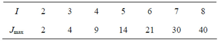
Table 1. Maximum number of sources.
minimal number of sensors is used to identify as many modes as possible.
The method is similar to that of [19], with the exception that the analytic signal is exploited. This leads to a reduction of the system order (to be identified) by a factor of two, reducing the required Hankel matrix size.
2. State Space System Preliminaries
Theoretical background on second-order and state-space systems is provided in this section. Consider the familiar second order Equation of Motion (EOM) for a linear system,
 (13)
(13)
Here  is the displacement vector for all DOF,
  is the force vector, B1 is the force influence matrix mapping the force vector to physical coordinates, M is the positive definite mass matrix, C is the positive semi-definite damping matrix and K is the positive semi-definite stiffness matrix. Matrices M, C and K are real valued and symmetric. Because K is positive semi-definite in general, the structure will have rigid body modes. However the rigid body modes and responses are generally not of interest in the modal identification problem. Therefore we will only consider oscillatory responses.
The second order EOM can be recast into a continuous-time state-space model,
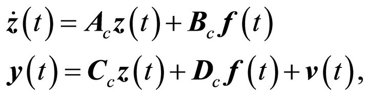 (14)
(14)
where  is the state vector,
  is the output vector and
  represents measurement noise. The plant,
  , input influence,
  output influence,
  ,and direct feedthrough,
  , matrices are given by:
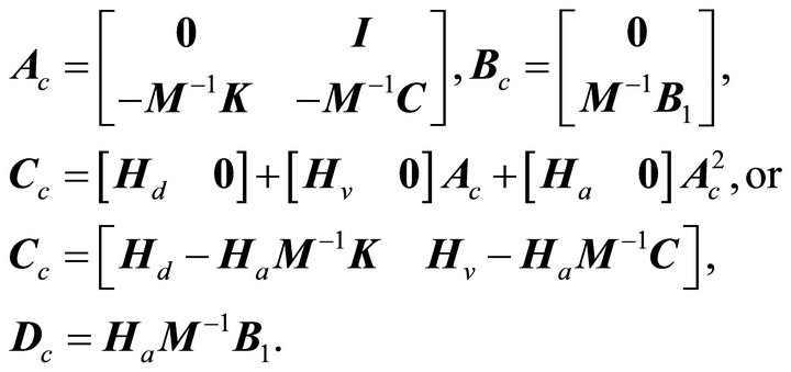 (15)
(15)
The permutation matrices Hd, Hv and Ha, contain rows with a single unit element with all other elements null, such that they pick-off the measured DOF. As an example, for acceleration sensing at all DOF,  , and
, and .
.
The set of differential equations can be decoupled using the transformation,  , where,
  is the matrix of eigenvectors of the plant matrix and
 is the modal state vector.
The matrix  takes the form,
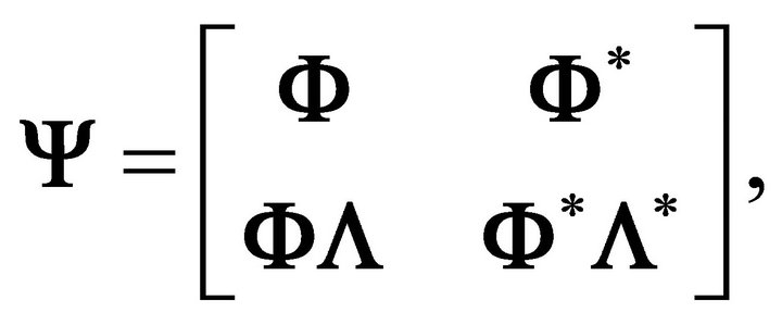 (16)
(16)
where  is the matrix of complex-valued system mode shapes,
  is the diagonal matrix of independent (not including conjugate pairs) plant matrix eigen values, and the symbol
  represents the complex conjugate. The diagonal system is given by:
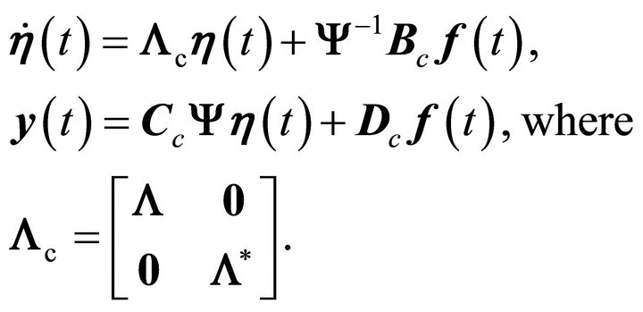 (17)
(17)
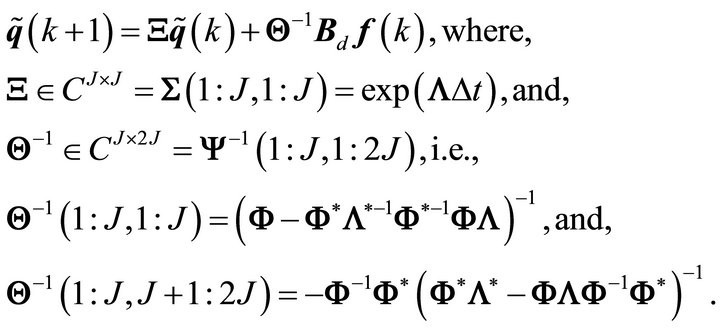
The continuous-time state-space system can be transformed into a discrete-time system with sampling interval Δt by:
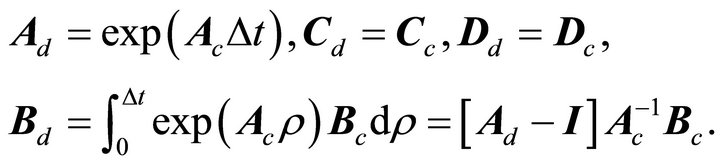 (18)
(18)
The transformation results in the discrete-time system,
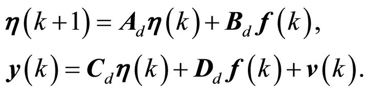 (19)
(19)
The set of difference equations can be decoupled through the transformation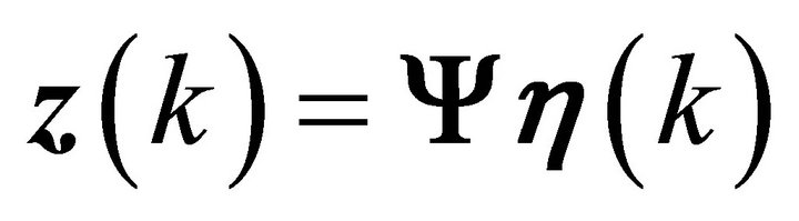 , yielding,
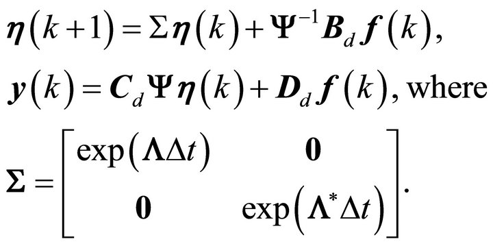 (20)
(20)
It was shown in [18,19] that for τ sufficiently large (compared to the decay rate of the force and noise correlation functions), the correlation matrices take the form,
 (21)
(21)
as terms involving the random input force and measurement noise dissipate quickly with increasing time shift, τ. The matrix  is the correlation of the state-space modal responses (at zero time shift). Reference [19] provided the proof that
  is diagonal if and only if the system is conservative, i.e., there is no system damping. The relative magnitude of the off diagonal terms can be significant when damping is present. It can also be seen from (21) that nondiagonality of
  causes
  to be nonhermetian for
 .
.
Equation (21) can be compared directly to the JAD problem solved in SOBI (6). In SOBI, it is assumed that the data correlation matrices,  , are Hermetian for all τ and, therefore, the right diagonalizing matrix factor is the Hermetian transpose of the left. In fact the nonhermetian part of the correlation matrices is discarded before application of Hermetian JAD. This leads to errors in the estimated mode shapes and modal responses when SOBI is applied. Windowing the data prior to application of SOBI alleviates this, as the correlation matrices of the windowed data are nearly Hermetian and the windowed modal correlation matrix is nearly diagonal, [6]. Diagonalization of the nonwindowed correlation matrices,
  , is preferred but requires separate left and right matrix factors.
3. Additional Preliminaries
In this section, additional developments are provided that set the stage for the BMIDHM algorithm.
3.1. Uniqueness of the Nonhermetian Diagonalization
Diagonalization of nonhermetian correlation matrices with separate left and right matrix factors, as in (21), is essential to estimate accurate modal parameters, while avoiding windowing the data set. However, it is known that such a diagonalization of a single correlation matrix is not unique. Consider, for example, that a single correlation matrix can be diagonalized by left and right singular vectors or left and right eigenvectors. Further to this point, an alternate set of left and right matrix factors can be derived that diagonalize  to the set of arbitrary diagonal matrices
 ,
,
 (22)
(22)
Here M is an arbitrary invertible matrix and the diagonalization holds when N can be found satisfying the prescribed relationship between N and M. If we consider a single value of , N can easily be obtained. However for multiple values of τ, a matrix N cannot generally be found that satisfies the above equation for all τ. Therefore the decomposition is unique for all practical purposes.
3.2. Analytic State-Space Form
In this section the analytic state-space form will be derived considering acceleration sensing. Forms for displacement and velocity sensing are similar. The output equation in (20) with acceleration sensing can be written as,
 (23)
(23)
If the redundant conjugate pairs are removed the first term becomes, . Recalling that the modal responses can be written as analytic signals, [9], and constructing the analytic signals of output, force and measurement noise, the analytic state-space output equation is arrived at,
 (24)
(24)
In (24), a tilde has been placed over the modal responses,  , to remind the reader that they are analytic signals. It should be noted that though the modal responses are analytic signals for free response and impulse response cases, they are not strictly analytic signals in the general forced response case. In the case of random excitation however, modal responses are analytic up to a random additive term, which does not affect the cross-correlation functions. The true modal responses can then be substituted by their corresponding analytic signals for modal identification purposes.
The state equation can also be written with redundant conjugate pairs removed, yielding the analytic state equation,
 (25)
(25)
In Equation (25), Matlab® notation is used for row and column partitions of a matrix. It can be seen from (25) that the analytic state-space system order is J, while representing the same dynamics as the original state-space system of (20) with order 2J. This proves advantageous for modal identification, as the desired system order is reduced by half, requiring smaller Hankel matrix size to identify the desired number of modes. The analytic, discrete-time, state-space form can be summarized as,
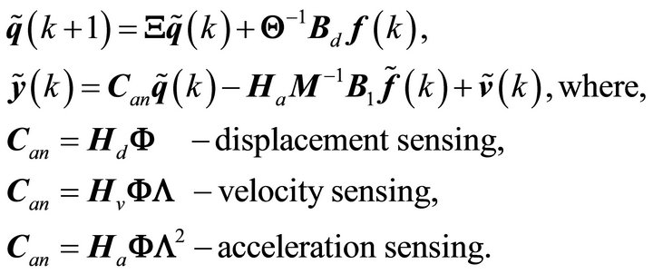 (26)
(26)
Note that in all cases,  consists of row partitions of scaled mode shapes. (Recall from properties of eigenvectors that mode shapes scaled by arbitrary complexvalued constant are still mode shapes.)
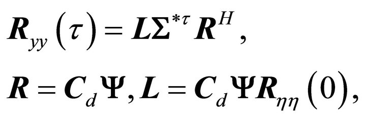
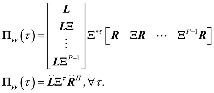
The correlation functions for sufficiently large τ can be written as,
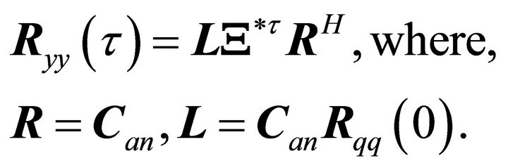 (27)
(27)
In (27), the right and left matrix factors, R and L respectively, have been redefined.
4. The BMIDHM Algorithm
The BMIDHM algorithm is derived in this section. The analytic signal of measured responses is first constructed by adding the Hilbert transform as the imaginary part,
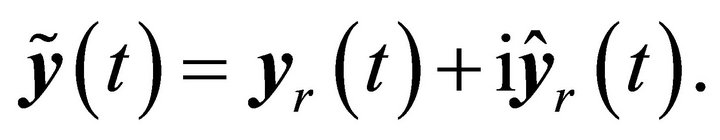 (28)
(28)
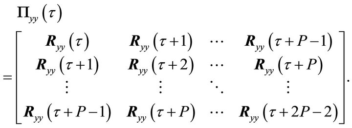
A set of K Hankel matrices, 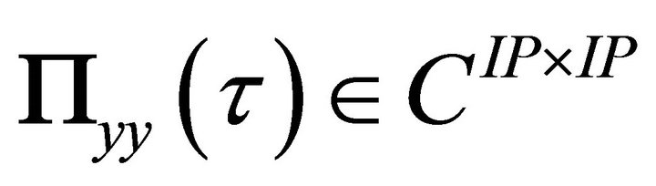 , is assembled, whereby the block elements are the correlation matrices of the analytic response data,
 (29)
(29)
Here, τ is the time shift operator and P is the number of block rows and columns in the Hankel matrix.
Nonhermetian JAD is applied to the set of Hankel matrices, yielding the decomposition,
 (30)
(30)
The fast-converging nonhermetian JAD algorithm of [20] was chosen for the decomposition. The algorithm results in the matrices ![]() and
and  directly, as opposed to the algorithm suggested in [19], which results in their generalized inverses, necessitating an additional inversion step.
Note that dimensions of![]() ,
,  and
and  are
are ,
,  , and
, and , respectively, where J is the system order,
 . The mode shapes (Can matrix) are obtained as the first J rows of
 . In practice, the system order may be ascertained by comparing the magnitudes of the diagonal elements of
 .
.
It was shown that by decomposing the Hankel matrices, up to IP complex modes can be identified. Because the analytic state-space form is used, the redundant complex conjugate modes are not included in the dynamics and are not identified in the decomposition. Therefore, all IP modes represent independent system modes (no conjugate pairs), as opposed to the method of [19], where they represent the independent modes and the complex-conjugate pairs. Summarizing, a necessary condition for identifying all J modes in the proposed methodology is , whereas the condition of [19] is
 .
.
The approximately diagonal plant matrices can be recovered for any τ by inverting (30),
 (31)
(31)
A set of T samples of the modal auto-correlation functions can then be taken from the diagonal elements of,
 (32)
(32)
Since only the diagonal elements of  are desired, and
  is diagonal, the matrix
  can be omitted without loss of generality. This is due to the fact that the diagonal elements of
  are simply equal to the diagonal elements of
  scaled by the diagonal elements of
 . Therefore the modal auto-correlation functions can be obtained by,
 (33)
(33)
Samples of the modal responses can be estimated by,
 (34)
(34)
where . The estimates will contain random noise due to neglecting the random force (if sensors are near input locations) and measurement noise terms in (34). If P is large enough, however, random force and noise terms average out.
A least squares estimate of the plant matrix,  , can be obtained by,
 (35)
(35)
Note that the estimated discrete-time plant and output influence matrices will approximately be in state-space modal coordinates, i.e.,  is approximately diagonal. Discrete time eigenvalues can be obtained as the eigenvalues of
 , and, can be converted to continuous time eigen-values by,
 (36)
(36)
Here,  is the operator that computes the eigen-values of a matrix. Natural frequencies, ωn, and modal damping ratios, ζj, can be recovered through the relation,
Alternatively, the natural frequencies and modal damping ratios can be computed from the modal correlation functions using simple SDOF methods.
5. Application to Simulation and Measured Data
In this section, results from application of the BMIDHM algorithm to simulated and measured data are presented. In each case the number of sensors utilized in the data set is kept low to evaluate the capabilities of the method when applied to the under determined problem.
5.1. Simulated 6 DOF System with Two Sensors
In order to investigate the effectiveness of the BMIDHM method, a six DOF mass-spring-dashpot system with non-diagonal damping was constructed. Three of the six DOF were chosen as sensor locations . The system was excited by uncorrelated, Gaussian-random, white noise applied to each of the six DOF. White noise was added to the response data with RMS equal to 10% of the maximum RMS among the response DOF. Figure 1 illustrates the displacement response along with the Fast Fourier Transform (FFT) of the displacement at each of the sensor locations.
The BMIDHM algorithm was applied to the measured data, selecting . The modal parameters (natural frequencies, modal damping ratios and mode shapes) of the six identified modes are compared to modal parameters of the six analytical modes in Table 2. Mode shapes are compared using a correlation coefficient known as the Modal Assurance Criterion (MAC), [21]. The MAC value between two modes
  and
and  is given by,
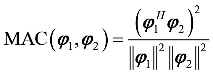 . (37)
A value near 1 indicates a good shape correlation. A value near 0 indicates poor correlation.
It can be seen that natural frequency and mode shape estimates compare extremely well, while the estimated modal damping ratios exhibit slightly more error. The modal auto-correlation functions and their FFTs, which are the power spectral densities, are shown in Figures 2 and 3. The shape observed in both the time domain and frequency domain indicates that the modes are completely isolated.
5.2. Simulated 4-Story Building Vibration
A model of a four story building was created by the University of British Columbia (UBC) as a benchmark for damage detection. In this section, modal identification of the undamaged structure with asymmetric floor mass is considered. The analytical model of a four story building mockup was modeled with Euler frame elements. The
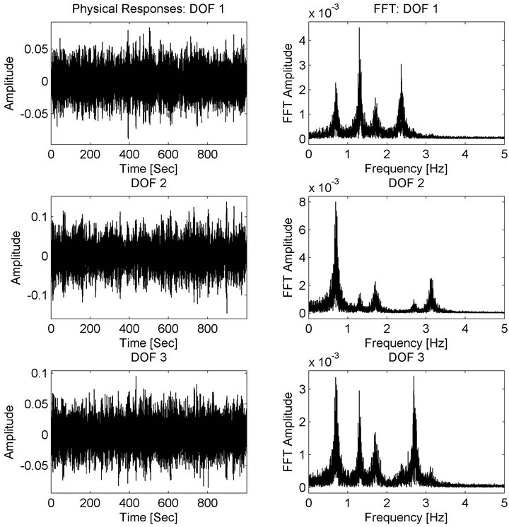
Figure 1. 6 DOF simulation-measured responses.

Table 2. 6 DOF simulation-modal parameters.
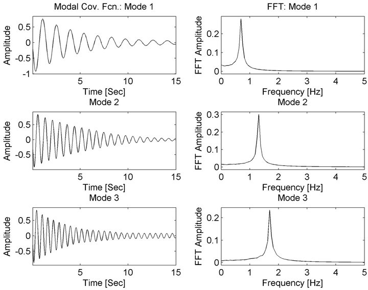
Figure 2. 6 DOF simulation-estimated modal response covariance functions 1 - 3.
FEM model with node numbering is shown in Figure 4.
The floors in the mockup are fairly rigid. Notice that
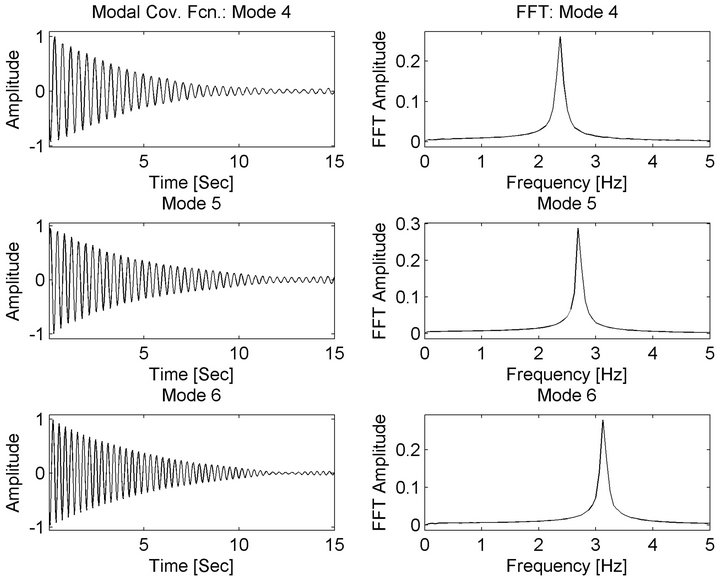
Figure 3. 6 DOF simulation-estimated modal response covariance functions 4 - 6.
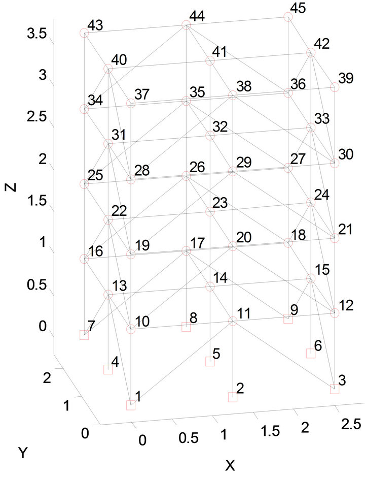
Figure 4. UBC building-FEM model.
the FEM model does not include explicit models for each floor. Instead, a rigidizing constraint was applied to the stiffness matrix as an ad-hoc step before simulation. For simulation, 1% diagonal-damping is applied in the modal domain. The resulting model contained 120 DOF. Note that the modeling and simulation was done in a MATLAB® package provided by the UBC.
The structure was excited in the transverse direction by a simulated diagonally oriented shaker at the top center of the building. Gaussian random excitation, filtered between 0 - 100 Hz was applied for 150 seconds. The time interval for integration was 0.001 seconds. Accelerations were measured at 16 locations. A pair of planar accelerometers was simulated on each floor, adjacent to the center columns by outputting x and y accelerations at nearby nodes. Measurement noise was simulated by adding Gaussian random noise to each measurement. The RMS of the noise was selected as 10% of the RMS of the measurement with the highest response level.
A plot of the Complex Mode Indicator Function (CMIF) is shown in Figure 5. The influence of 11 modes on the response shape can be seen as well as the additive measurement noise. Note that the first two modes are closely spaced modes (~9 Hz) representing the first sway modes in the x and y directions. The poorly excited third mode (~14 Hz) is the first torsional mode. The influence of many frequencies on the response shape can be seen as well as the additive measurement noise. Due to these characteristics, this data set presents a challenge to the BMIDHM algorithm. Data from five of the 16 available sensors were chosen as the data set .
.
Modal identification was performed on the response data (ignoring the input force data) using BMIDHM, selecting . Two noise modes were separated out based on the poor spectral and temporal shape of the identified modal responses and low contribution to the vibration response. The modal parameters of the remaining 11 modes are compared to modal parameters of the 11 analytical modes in Table 3. Note that the frequency
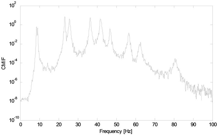
Figure 5. UBC building simulation-first CMIF.
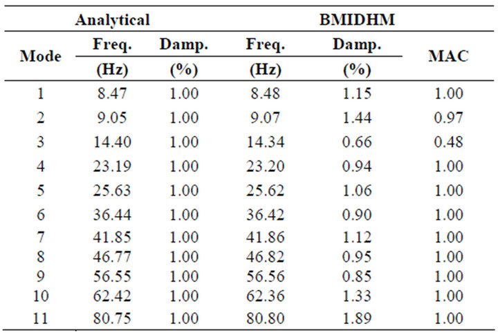
Table 3. UBC building simulation-modal parameters.
and damping results for mode 3 were obtained by SDOF fitting methods using data around the peaks of the modal spectra. It can be seen that natural frequency and mode shape estimates compare well, but estimated modal damping ratios tend to have more error.
Modal response auto-correlation functions and their FFTs are shown in Figures 6-8. The shape observed in both the time domain and frequency domain indicates that the modes are completely isolated for all modes except for the third. A peak in the spectrum is visible for the poorly-excited third mode at the correct frequency of 14.35 Hz, however another large peak is present as well as a high noise level above 30 Hz. Bandpass filtering the data from 10 - 20 Hz results in improved spectral and temporal shape (Figure 9).
5.3. Heritage Court Tower Building
The structure analyzed in this section is the Heritage Court Tower (HCT) building. The description of the building, provided in [22] is summarized here. The HCT is located in downtown Vancouver, British Columbia, Canada. It is a 15-story reinforced concrete shear core building. The building is essentially rectangular in shape with only small projections and setbacks. The building tower is short and stout, having a height to width aspect ratio of approximately 1.7 in the east-west direction and

Figure 6. UBC building simulation-estimated modal response covariance functions 1 - 4.
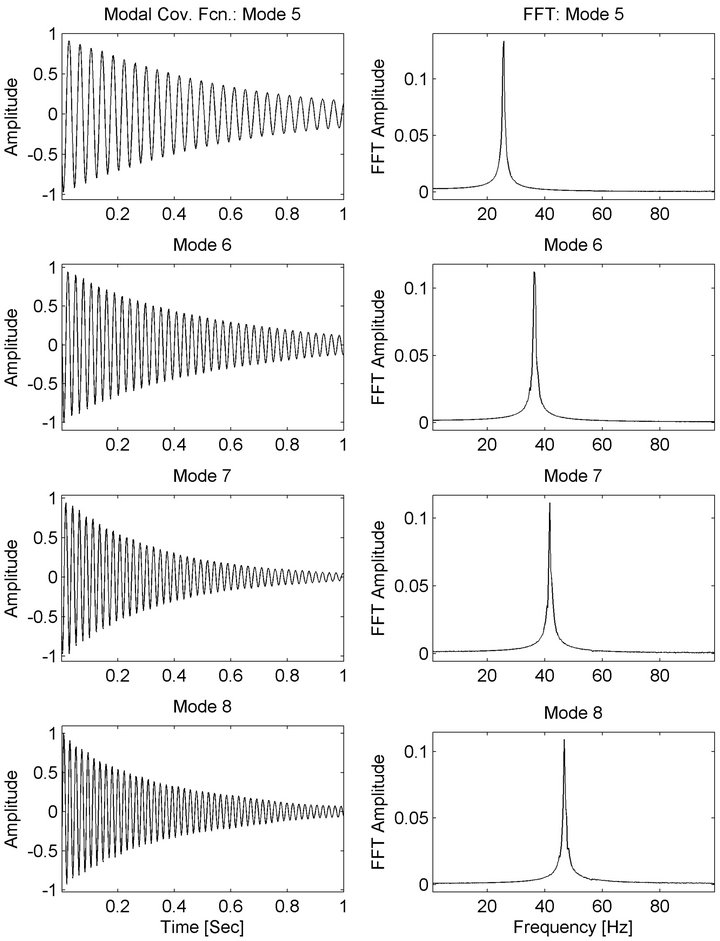
Figure 7. UBC building simulation-estimated modal response covariance functions 5 - 8.
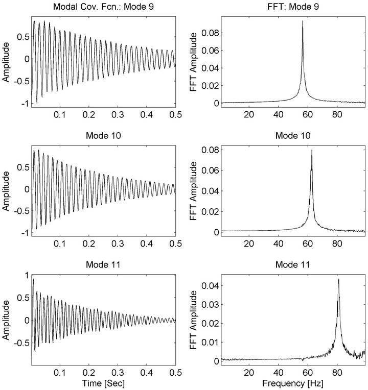
Figure 8. UBC building simulation-estimated modal response covariance functions 9 - 11.
1.3 in the north-south direction. An overview of the building is presented in Figure 10. Typical floor dimensions of the upper floors are about 25 meters by 31 me-

Figure 9. UBC building simulation-estimated modal response covariance functions 3 (Filtered).

Figure 10. Photograph of Heritage Court Tower (HCT) building.
ters, while the dimensions of the lower three levels are about 36 meters by 30 meters. The footprint of the building below ground level is about 42 meters by 36 meters. The height of the first story is 4.7 meters, while most of the other levels have heights of 2.7 meters. Elevator and stairs corridors are concentrated at the center core of the building and form the main lateral resisting elements against potential wind and seismic lateral and torsional forces. The tower structure sits on top of four levels of reinforced concrete underground parking. A parking structure extends approximately 14 meters beyond the tower in the south direction forming an L-shape with the tower. The parking structure and first floors of the tower are fairly flush on the remaining three sides. Because the building sits to the north side of the underground parking structure, coupling of the torsional and lateral modes of vibration was expected primarily in the EW direction.
Four sets of ambient response data were collected with eight accelerometers. Six of the accelerometers were roving transducers that changed location for each data set. Two reference accelerometers remained in a fixed location. This enables the mode shapes computed from the four data sets to be combined into one modal matrix. The data sets contained around 325 seconds of data, sampled at 40 Hz.
The third data set was analyzed using BMIDHM as well as the state-space realization method, known as covariance-driven Stochastic Subspace Identification (SSI). Covariance-driven SSI is essentially an application of ERA on cross-correlation functions instead of impulse response functions. More details of the SSI algorithm can be found in [23]. Channels 2, 4, 7 and 8 were chosen as reference channels for SSI. The BMIDHM and SSI methods were applied on the ambient responses directly.
The first two Complex Mode Indicator Functions (CMIFs) are shown in Figure 11. From the CMIF plot, it can be seen that the first three modes are closely spaced. In fact the first two modes (~1.25 Hz) are so closely spaced that they are nearly the same frequency. As a result, the first CMIF does not exhibit two distinct peaks. However the presence of the second mode at ~1.25 Hz is indicated by the peak in the second CMIF. There is a sharp peak in the first CMIF around 8.7 Hz. This is most likely harmonic noise due to a mechanical device such as a motor, fan or pump. Also notice that above 10 Hz, there are no distinct peaks visible. This data set presents a challenge to the BMID method due to the small number of sensors, presence of closely spaced modes and the presence of noise.
In order to evaluate the capabilities of BMIDHM for the underdetermined problem, the frequency band from
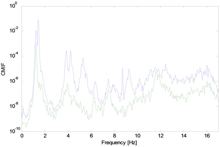
Figure 11. HCT building—The first two CMIFs.
0.0 - 7.5 Hz is focused on, only three of the eight available sensors are chosen . All eight sensors are used in the SSI algorithm so that results from BMIDHM can be compared to an accurate set of modal parameters. Modal identification was performed on the ambient response data using BMIDHM, selecting
 . Three noise modes were discarded based on the poor spectral and temporal shape of the identified modal responses and low contribution to the vibration response.
The SSI method was performed with several different Toeplitz matrix sizes, resulting in several realizations. Consistency diagrams were formed for each filter band, and the best realization was chosen. The consistency diagrams can be found in [8].
Modal parameters from the two methods are presented in Table 4. Modal parameters from BMIDHM applied using three sensors compare quite will to those obtained using SSI applied on all eight sensors, though damping error is significant for some modes.
Modal auto-correlation functions from the BMIDHM method are shown in Figures 12 and 13. Note that the time scale is different in the two figures. The FFTs of the random modal responses computed using (34) are provided in Figure 14. The modal response autocorrelation functions exhibit clean, monotone decay and the spectral peaks are seen to be quite well-separated in the modal responses and modal auto-correlations.
6. Conclusions
Methods employed in state-space realization theory and second order blind source separation were combined, formulating an new modal identification algorithm. The algorithm is applied on measured vibration (output-only) data and results in estimates of the system:
complex-valued modal matrix;
modal responses and auto-correlation functions (even in the underdetermined case);
state-space discrete-time plant, output-influence and observability matrices in modal form;
natural frequencies and fractions of modal damping.
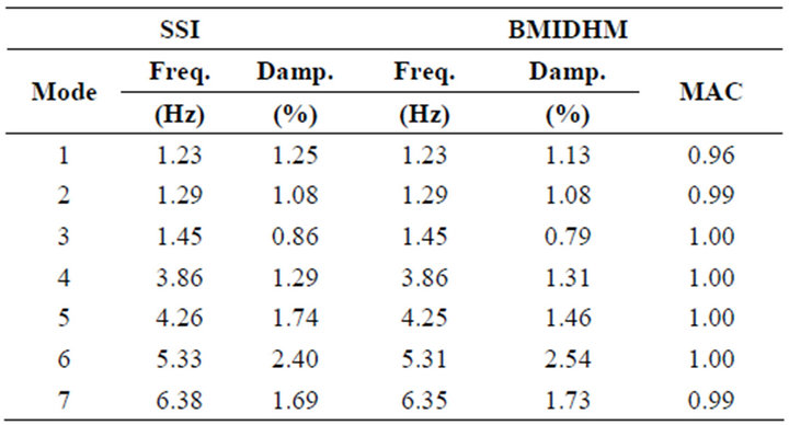
Table 4. HCT building simulation-modal parameters.
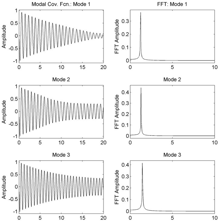
Figure 12. hct building-estimated modal response covariance functions 1 - 3.
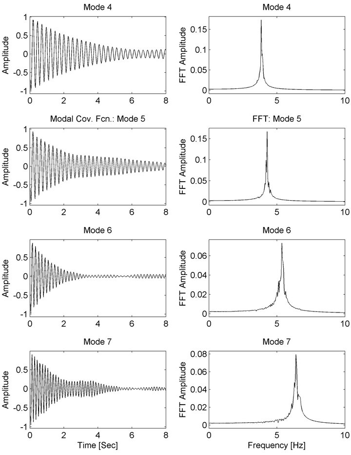
Figure 13. HCT building-estimated modal response covariance functions 4 - 7.
Compared to the first practical adaptation of BSS to modal identification, [6], several improvements can be cited:
The whitening, windowing and pairing routines are
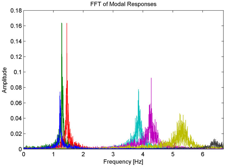
Figure 14. HCT building-FFT of estimated modal responses.
precluded.
Application to the underdetermined problem (more independent modes than sensors) is effectively handled, resulting in high-quality modal parameters, modal auto-correlation functions and modal responses with few sensors.
The state-space plant matrix and corresponding system eigenvalues are readily available.
REFERENCES
- L. Tong, V. C. Soon, Y. Huang and R. Liu, “AMUSE: A New Blind Identification Algorithm,” Proceedings of IEEE International Symposium on Circuits and Systems, New Orleans, 1-3 May 1990, pp. 1784-1787. doi:10.1109/ISCAS.1990.111981
- A. Belouchrani, K. Abed-Meraim, J.-F. Cardoso and E. Moulines, “A Blind Source Separation Technique Using Second-Order Statistics,” IEEE Transactions on Signal Processing, Vol. 45, No. 2, 1997, pp. 434-444. doi:10.1109/78.554307
- S. Chauhan, R. J. Allemang, R. Martell and D. L. Brown, “Application of Independent Component Analysis and Blind Source Separation Techniques to Operational Modal Analysis,” Proceedings of the 25th International Modal Analysis Conference, Orlando, 19-22 February 2007.
- F. Poncelet, G. Kerschen, J.-C. Golinval and D. Verhelst, “Output-Only Modal Analysis Using Blind Source Separation Techniques,” Mechanical Systems and Signal Processing, Vol. 21, No. 6, 2007, pp. 2335-2358. doi:10.1016/j.ymssp.2006.12.005
- W. Zhou and D. Chelidze, “Blind Source Separation Based Vibration Mode Identification,” Proceedings of the 25th International Modal Analysis Conference, Orlando, 19-22 February 2007, pp. 3072-3087.
- S. I. McNeill and D. C. Zimmerman, “A Framework for Blind Modal Identification Using Joint Approximate Diagonalization,” Mechanical Systems and Signal Processing, Vol. 22, No. 7, 2007, pp. 1526-1548. doi:10.1016/j.ymssp.2008.01.010
- S. I. McNeill, “Modal Identification Using Blind Source Separation Techniques,” Ph.D. Dissertation, University of Houston, Houston, 2007.
- S. I. McNeill and D. C. Zimmerman, “Blind Modal Identification Applied to Output-Only Building Vibration,” Proceedings of the 28th International Modal Analysis Conference, Jacksonville, 2010.
- S. I. McNeill, “An Analytic Formulation for Blind Modal Identification,” Journal of Vibration and Control, Vol. 18, No. 14, 2012, pp. 2111-2121. doi:10.1177/1077546311429146
- A. Belouchrani, K. Abed-Meraim, J.-F. Cardoso and E. Moulines, “A Blind Source Separation Technique Using Second-Order Statistics,” IEEE Transactions on Signal Processing, Vol. 45, No. 2, pp. 434-444. doi:10.1109/78.554307
- P. Tichavsky and A. Yeredor, “Fast Approximate Joint Diagonalization Incorporating Weight Matrices,” IEEE Transactions of Signal Processing, Vol. 57. No. 3, 2009, pp. 878-891. doi:10.1109/TSP.2008.2009271
- P. Tichavsky, A. Yeredor and J. Nielsen, “A Fast Approximate Joint Diagonalization Algorithm Using a Criterion with a Block Diagonal Weight Matrix,” Proceedings of the 2008 International Conference on Acoustics, Speech and Signal Processing, Las Vegas, 31 March-4 April 2008, pp. 3321-3324.
- P. Tichavsky, “UWEDGE_C—Complex Version (Version for Complex-Valued Matrices and Complex-Valued Mixing) of the Algorithm UWEDGE,” 2010. http://si.utia.cas.cz/downloadPT.htm
- F. Abazarsa, S. Ghahari, F. Nateghi and E. Taciroglu, “Response-Only Modal Identification of Structures Using Limited Sensors,” Structural Control and Health Monitoring, Vol. 20, No. 6, 2013, pp. 987-1006. doi:10.1002/stc.1513
- F. Abazarsa, S. Ghahari, F. Nateghi and E. Taciroglu, “Blind Modal Identification of Non-Classically Damped Systems from Free or ambient Vibration Records,” Earthquake Spectra, in Press.
- S. I. McNeill, “Extending Blind Modal Identification to the Underdetermined Case for Ambient Vibration,” Proceedings of the ASME 2012 International Mechanical Engineering Congress & Exposition, Houston, 9-15 November 2012.
- L. De Lathauwer and J. Castaing, “Blind Identification of Underdetermined Mixtures by Simultaneous Matrix Diagonalization,” IEEE Transactions on Signal Processing, Vol. 56, No. 3, 2008, pp. 1096-1105. doi:10.1109/TSP.2007.908929
- J. Antoni and S. Chauhan, “Second Order Blind Source Separation Techniques (SO-BSS) and Their Relation to Stochastic Subspace Identification (SSI) Algorithm,” Pro- ceedings of the 28th International Modal Analysis Conference (IMAC), 2010.
- J. Antoni and S. Chauhan, “A Study and Extension of Second-Order Blind Source Separation to Operational Modal Analysis,” Journal of Sound and Vibration, Vol. 332, No. 4, 2013, pp. 1079-1106. doi:10.1016/j.jsv.2012.09.016
- A.-J. van der Veen, “Joint Diagonalization via Subspace Fit- ting Techniques,” International Conference on Acoustics, Speech, and Signal Processing—ICASSP, Salt Lake City, 7-11 May 2001, pp. 2773- 2776.
- R. J. Allemang and D. L. Brown, “A Correlation Coefficient for Modal Vector Analysis,” Proceedings of the 1st International Modal Analysis Conference, Orlando, 8-10 November 1982, pp. 110-116.
- C. Ventura, R. Brinker, E. Dascotte and P. Anderson “FEM Updating of the Heritage Court Building Structure,” Proceedings of the 19th International Modal Analysis Conference, Kissimmee, 5-8 February, 2001, pp. 324- 330.
- B. Peeters, “System Identification and Damage Detection in Civil Engineering,” Ph.D. Dissertation, Katholike Universite Leuven, Belgium, 2000.