Journal of Signal and Information Processing
Vol.3 No.1(2012), Article ID:17686,8 pages DOI:10.4236/jsip.2012.31014
An Improved Image Denoising Method Based on Wavelet Thresholding
![]()
Department of Computer Science & Engineering, Indian School of Mines, Dhanbad, India.
Email: {hariom4india, mantoshb}@gmail.com
Received November 10th, 2011; revised December 13th, 2011; accepted December 25th, 2011
Keywords: Wavelet Transforms; Neighboring Coefficients; Wavelet Thresholding; Image Denosing; Neighbouring Coefficients; Peak Signal-to-Noise Ratio
ABSTRACT
VisuShrink, ModineighShrink and NeighShrink are efficient image denoising algorithms based on the discrete wavelet transform (DWT). These methods have disadvantage of using a suboptimal universal threshold and identical neighbouring window size in all wavelet subbands. In this paper, an improved method is proposed, that determines a threshold as well as neighbouring window size for every subband using its lengths. Our experimental results illustrate that the proposed approach is better than the existing ones, i.e., NeighShrink, ModineighShrink and VisuShrink in terms of peak signal-to-noise ratio (PSNR) i.e. visual quality of the image.
1. Introduction
An image is often corrupted by noise during its acquisition and transmission. Image denoising is used to remove the additive Gaussian noise while retaining important maximum possible image features. Wavelet analysis has been demonstrated to be one of the powerful methods for performing image noise reduction [1,2]. The procedure for noise reduction is applied on the wavelet coefficients obtained after applying the wavelet transform to the image at different scales. The motivation for using the wavelet transform is that it is good for energy compaction since the small and large coefficients are more likely due to noise and important image features, respectively [3]. The small coefficients can be thresholded without affecting the significant features of the image. In its most basic form, each coefficient is thresholded by comparing against a value, called threshold. If the coefficient is smaller than the threshold, it is set to zero; otherwise it is kept either as it is or modified. The inverse wavelet transform on the resultant image leads to reconstruction of the image with essential characteristics [4].
Since the pioneer work of Donoho & Johnstone, there have been many works on finding suitable thresholds; however, very few have been designed for images [4-6]. There exist various methods for wavelet thresholding which rely on the choice of a threshold value such as VisuShrink [5,7], SureShrink [4,8] and BayesShrink [9]. The VisuShrink [5] has a limitation of not dealing with minimizing the mean squared error, i.e. it removes too many coefficients. However, it is known to give the recovered images that are overly smoothed. The SureShrink threshold depends upon Stein’s Unbiased Risk Estimator (SURE) [7]. It minimizes the mean squared error that takes the combination of the universal threshold and the SURE threshold. In this method, the employed thresholding is adaptive, i.e., if the unknown function contains abrupt changes or boundaries in the image, the reconstructed image also does. The BayesShrink [9] is a data-driven adaptive image denoising method. Hall et al. and Cai studied local block thresholding rules for wavelet function estimation [10-12]. These methods threshold the empirical wavelet coefficients in groups rather than individually, making simultaneous decisions to retain or to discard all the coefficients within non-overlapping blocks. The proposed method overcomes the limitations of the above mentioned methods. It determines the threshold and neighbouring window size for every subband using its lengths.
The rest of the paper is organized as follows. Section 2 describes the related work. Section 3 discusses the proposed work. The experimental results are given in Section 4. The results are discussed by taking three test images and various noise levels. Finally, the concluding remarks are given in Section 5.
2. Related Work
The VisuShrink method, introduced by Donoho [5], uses a threshold value T that is proportional to the standard deviation of the noise. It follows the hard thresholding rule. The threshold in VisuShrink is also referred to as universal threshold and it is defined as:
where σ is the noise variance present in the signal and M represents the signal size or number of samples.
An estimate of the noise level σ is defined based on the median absolute deviation that is given by:

where  subband.
A threshold chosen based on Stein’s Unbiased Risk Estimator (SURE) [4,8] is called as SureShrink. It is a combination of the universal threshold and the SURE threshold. This method specifies a threshold value tj for each resolution level j in the wavelet transform which is referred to as level dependent thresholding. The goal of SureShrink is to minimize the mean squared error that is defined as:
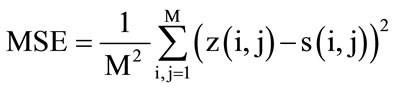 where z(x, y) is the estimate of the image and s(x, y) is the original image without noise and M × M is the image size. The SureShrink suppresses the noise by thresholding the empirical wavelet coefficients. The SureShrink threshold t* is defined as:
where t denotes the value that minimizes Stein’s Unbiased Risk Estimator, σ is the noise variance, and M is the size of the image. SureShrink follows the soft thresholding rule. The thresholding employed in this case is adaptive, i.e., a threshold level is assigned to each dyadic resolution level by the principle of minimizing the Stein’s Unbiased Risk Estimator for threshold estimates.
The BayesShrink [9] minimizes the Bayesian risk, and hence its name, BayesShrink. It uses soft thresholding and is subband-dependent, which means that the thresholding is done at each band of resolution in the wavelet decomposition. Like the SureShrink procedure, it is smoothness-adaptive. The Bayes threshold, tB, is defined as:
where σ2 is the noise variance and σs is the signal variance without noise. The noise variance σ2 is estimated from the subband HH1.
The aim of local thresholding rules is to increase the estimation accuracy by utilizing information about neighboring wavelet coefficients. The block thresholding increases the estimation precision by utilizing the information about the neighbor wavelet coefficients. Recently, there has been a fair amount of research to select the threshold for image denoising from the noisy image using wavelet [13-16].
The choice of a threshold is an important point of interest. It plays a major role in noise removal of images because denoising most frequently produces smoothed images, reducing their sharpness. Generally, the choice should be taken to preserve the edges of the denoised image. Our proposed image denoising method is based on thresholding that not only removes noise but also preserves the edges. It is discussed in next section.
3. Proposed Work
Before discussing our proposed work, we will review the wavelet transform in brief.
Let x = {x(i, j), i, j = 1, 2, ···, M} denote M × M original image to be recovered and M is some integer power of 2. During transmission, the image x is corrupted by independent and identically distributed (i.i.d) zero mean, white Gaussian Noise, i.e. n(i, j) ~ M (0, σ2). At the receiver end, the noisy observations g(i, j)= x(i, j) + σ n(i, j) are obtained. The goal is to estimate x from the noisy observation g(i, j) such that the mean squared error (MSE) is minimum [3]. Let W and W-1 denote the two dimensional discrete wavelet transform (DWT) and its inverse (IDWT), respectively. Then Y = W * g represents the matrix of wavelet coefficients of g having four subbands (LL, LH, HL and HH) [17-19]. The subbands HH, HL, LH are called details and the subband LL is called approximation. Performing DWT on LL, we again get four subbands. We can perform DWT of approximation subband obtained in previous wavelet transform multiple times so that the final approximation band contains only single value. Denote the maximum number of levels (decompositions) by J. The size of the subband at scale k is M/2k × M/2k. Figure 1 shows two level decomposition of an image. The wavelet thresholding denoising method processes each coefficient Y(i, j) from the detail subbands with a threshold function to obtain . The denoised estimate
  of the image x is inverse wavelet transform of
 , i.e.,
 .
.
We now discuss the parameter estimation,
3.1. Parameters Estimation
(i) In our proposed method, we calculate threshold value TNEW using the following:
 (1)
(1)
where , here k = 1, 2, ···, J. J represents subband.
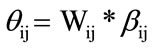
(ii) Let Wij be the wavelet coefficients of interest in the neighborhood window . Calculate
 :
:
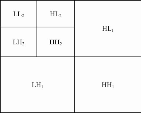
Figure 1. 2D-DWT with 2-Level decomposition.
 within the window
(iii) Shrink the wavelet coefficients by using:
(iv) The shrinkage factor is given as:
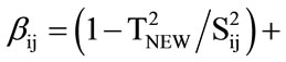
here “+” means that the positive value should be kept as it is and the negative value should be replaced by zero.
After apply this thresholding function and using NeighShrink, it was observed that the reconstructed image had mat like aberrations when the noise content was high. We could remove these aberrations using Wiener filter.
Using NeighShrink we loose some details of the image and sometimes the reconstructed image becomes unacceptably blurred. The reason of this blurring may be the suppression of too many details of wavelet coefficients. This problem can be avoided using the following shrinkage factor is:

3.2. Denoising Algorithm
The proposed procedure is given below:
• Perform multiscale decomposition on the image corrupted by Gaussian noise. The 2-D wavelet transform W on the noisy image Y is performed up to Jth level to generate several subbands.
• Estimate the robust median using the following:
 (2)
(2)
• For each level, compute TNEW as a threshold using (1).
• For each subband (except the low pass residual), apply NeighShrink method to obtain the noiseless wavelet coefficients.
• Perform the inverse wavelet transform on the modified coefficients to obtain the denoised estimate image .
.
4. Results and Discussions
We have evaluated the performance of our proposed method using the quality measure PSNR which is calculated as:
 where MSE is the mean squared error between the original image and reconstructed image.
Here, we have compared the performance of our scheme with different de-noising schemes that include Visushrink, NeighShrink and ModineighShrink. We have taken different window sizes of 2 × 2, 3 × 3, 5 × 5, and 7 × 7. The noise levels have been taken as 10, 20, 30, 50, 75, and 100. The images considered in our experiments are standard images that include Lena, Barbara, and Goldhill each of size 512 × 512 (refer Figure 2). The wavelet transform used is Daubechies least asymmetric compactly supported wavelet with eight vanishing moments [20]. We have performed wavelet transform four times in order to obtain four scales of decomposition.
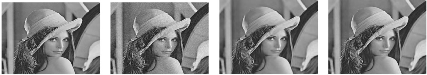
We have drawn graphs for PSNR vs noise level for the VisuShrink, NeighShrink, ModNeiSh and proposed methods for Lena image and they are shown in Figures 4(a)-(d), for window sizes 2 × 2, 3 × 3, 5 × 5 and 7 × 7, respectively. It is evident from these figures that our proposed method performs better than the VisuShrink, NeighShrink, ModNeiSh methods for all window sizes considered in this paper. The only case when our method performs no better then these methods is for window size of 7 × 7 and noise level up to 20. In fact, for higher values of noise, the performance of all methods converges as is evident from the Figures 4(a)-(d). The reason is that all the methods, remove almost same number of coefficients. For other two images, i.e., Barbara and Goldhill, similar graphs were obtained. We have shown in Figures 3(a)-(n) images of Lena using noise level 10 and different window sizes. Similar results were obtained for other images also. We however have given the numerical results for all images in Tables 1-4.
5. Conclusion
Our proposed scheme performs better for all noise levels and for all window sizes under consideration for PSNR
 (a)
(a) (b)
(b)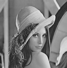 (c)
(c)
Figure 2. Original test images with 512 × 512 pixels: (a) Lena; (b) Barbara; (c) Goldhill.
 (a)
(a) (b)
(b) (c)
(c)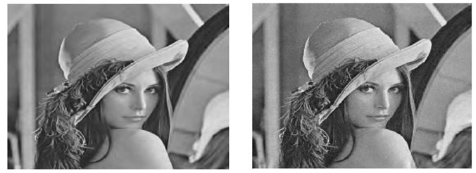 (d)
(d)
Figure 3. Comparative performance of various methods on Lena with noise level 10 (a) Original; (b) Noisy image with noise level 10; (c) Denoise using VisuShrink (3 × 3); (d) Denoise using VisuShrink (5 × 5); (e) Denoise using VisuShrink (7 × 7); (f) Denoise using NeighShrink (3 × 3); (g) Denoise using NeighShrink (5 × 5); (h) Denoise using NeighShrink (7 × 7); (i) Denoise using ModNeiSh (3 × 3); (j) Denoise using ModNeiSh (5 × 5); (k) Denoise using ModNeiSh (7 × 7); (l) Denoise using Proposed (3 × 3); (m) Denoise using Proposed (5 × 5); (n) Denoise using Proposed (7 × 7).
 (a)
(a)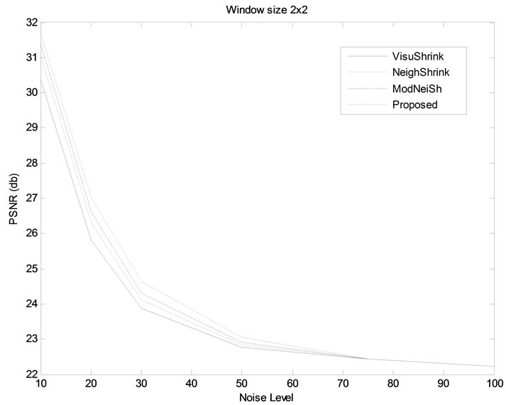 (b)
(b) (c)
(c) (d)
(d)
Figure 4. PSNR gain vs noise level of Proposed, VisuShrink, NeighShrink, ModineighShrink (ModNeiSh) methods for Lena image for window size. (a) 2 × 2; (b) 3 × 3; (c) 5 × 5; (d) 7 × 7.
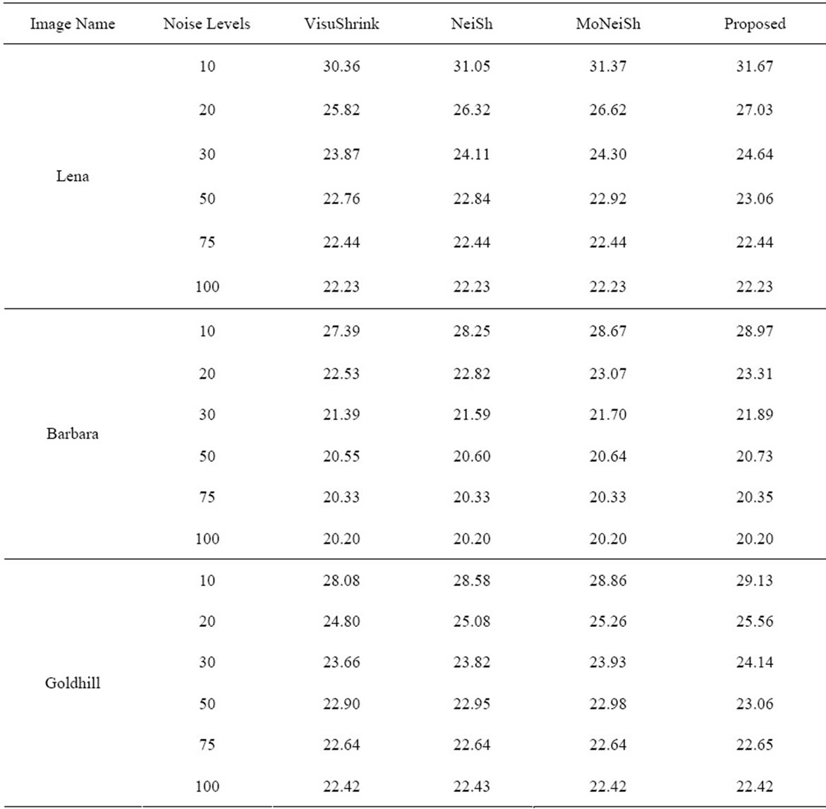
Table 1. Denoising results (PSNR in db) for Lena, Barbra and Goldhill using window size of 2 × 2.
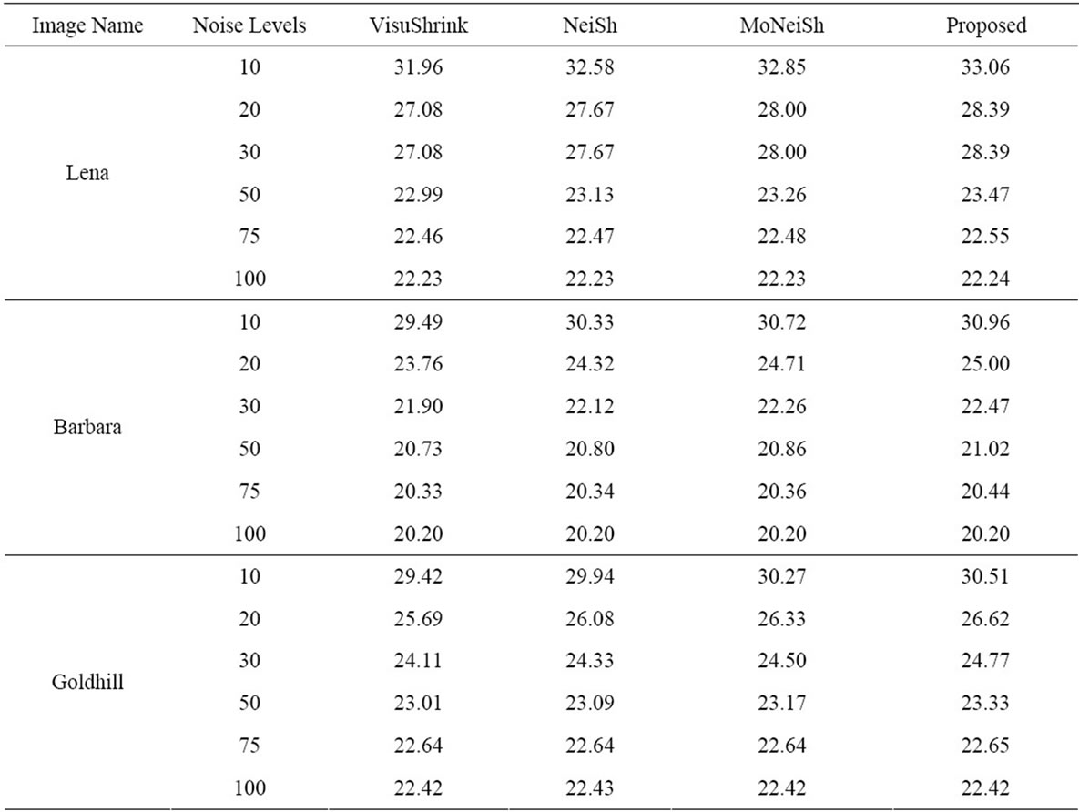
Table 2. Denoising results (PSNR in db) for Lena, Barbra and Goldhill using window size of 3 × 3.
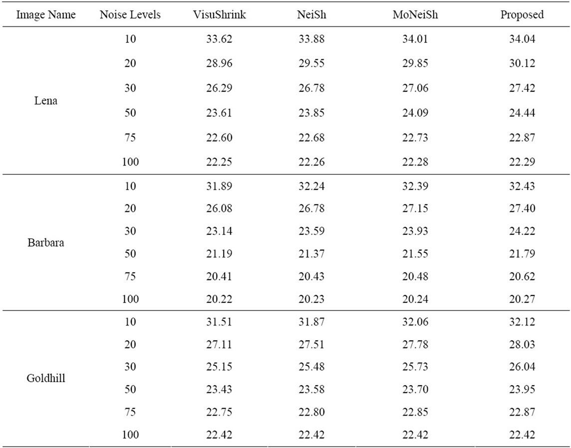
Table 3. Denoising results (PSNR in db) for Lena, Barbra and Goldhill using window size of 5 × 5.

Table 4. Denoising results (PSNR in db) for Lena, Barbra and Goldhill using window size of 7 × 7.
value and visual quality of the denoised image than Visushrink, NeighShrink and Modified NeighShrink for all window sizes and almost all noise levels.
6. Acknowledgements
The authors express their sincere thanks to Prof. S. Chand for his invaluable comments and suggestions.
REFERENCES
- C. S. Burrus, R. A. Gopinath and H. Guo, “Introduction to Wavelet and Wavelet Transforms,” Prentice Hall, New Jersey, 1997.
- S. Mallat, “A Wavelet Tour of Signal Processing,” 2nd Edition, Academic, New York, 1999.
- M. Jansen, “Noise Reduction by Wavelet Thresholding,” Springer-Verlag, New York, 2001. doi:10.1007/978-1-4613-0145-5
- D. L. Donoho and I. M. Johnstone, “Ideal Spatial Adaptation via Wavelet Shrinkage,” Biometrika, Vol. 81, No. 3, 1994, pp. 425-455. doi:10.1093/biomet/81.3.425
- D. L. Donoho, “De-Noising by Soft Thresholding,” IEEE Transactions on Information Theory, Vol. 41, No. 3, 1995, pp. 613-627. doi:10.1109/18.382009
- D. L. Donoho and I. M. Johnstone, “Wavelet Shrinkage: Asymptotic?” Journal of the Royal Statistical Society: Series B, Vol. 57, No. 2, 1995, pp. 301-369.
- D. L. Donoho and I. M. Johnstone, “Adapting to Unknown Smoothness via Wavelet Shrinkage,” Journal of American Statistical Association, Vol. 90, No. 432, 1995, pp. 1200-1224. doi:10.2307/2291512
- X. P. Zhang and M. D. Desai, “Adaptive Denoising Based on SURE Risk,” IEEE Signal Processing Letters, Vol. 5, No. 10, 1998, pp. 265-267. doi:10.1109/97.720560
- S. G. Chang, B. Yu and M. Vetterli, “Adaptive Wavelet Thresholding for Image Denoising and Compression,” IEEE Transactions on Image Processing, Vol. 9, No. 9, 2000, pp. 1532-1546. doi:10.1109/83.862633
- T. T. Cai and B. W. Silverman, “Incorporating Information on Neighboring Coefficients into Wavelet Estimation,” Sankhya Series B, Vol. 63, No. 2, 2001, pp. 127- 148.
- T. T. Cai, “Adaptive Wavelet Estimation, a Block Thresholding and Oracle Inequality Approach,” Annals of Statistics, Vol. 27, No. 3, 1999, pp. 898-924. doi:10.1214/aos/1018031262
- T. T. Cai and H. H. Zhou, “A Data-Driven Block Thresholding Approach to Wavelet Estimation,” Annals of Statistics, Vol. 37, No. 2, 2009, pp. 569-595. doi:10.1214/07-AOS538
- F. N. Yi, et al., “A Wavelet Threshold of a New Method of Image Denoising,” Science & Technology Information, 2008.
- S. Ruikar and D. D. Doye, “Image Denoising Using Wavelet Transform,” 2010 2nd International Conference on Mechanical and Electrical Technology, Singapore, 10-12 September 2010, pp. 509-515. doi:10.1109/ICMET.2010.5598411
- P. Hedaoo and S. S. Godbole, “Wavelet Thresholding Approach for Image Denoising,” International Journal of Network Security & Its Applications, Vol. 3, No. 4, 2011, pp. 16-21.
- V. Nigam, S. Luthra and S. Bhatnagar, “A Comparative Study of Thresholding Techniques for Image Denoising,” 2010 International Conference on Computer and Communication Technology, Allahabad, 17-19 September 2010, pp. 173-176.
- M. Vattereli and J. Kovacevic, “Wavelets and Subband Coding,” Prentice Hall, Englewood Cliffs, 1995.
- S. Gupta and L. Kaur, “Wavelet Based Image Compression Using Daubechies Filters,” Proceedings of the 8th National Conference on Communications, Bombay, 2002.
- M. J. T. Smith and S. L. Eddins, “Analysis/Synthesis Techniques for Sub Band Image Coding,” IEEE Transactions Acoustics, Speech and Signal Processing, Vol. 38, No. 8, 1990, pp. 1446-1456. doi:10.1109/29.57579
- I. Daubechies, “Ten Lectures on Wavelets,” Proceedings of the CBMS-NSF Regional Conference Series in Applied Mathematics, Philadelphia, Vol. 61, 1992.