International Journal of Geosciences
Vol.4 No.10(2013), Article ID:41524,13 pages DOI:10.4236/ijg.2013.410140
Spatial Interpolation of Tidal Data Using a Multiple-Order Harmonic Equation for Unstructured Grids
1Coast Survey Development Laboratory, NOAA, Silver Spring, USA
2Earth Resources Technology, Laurel, USA
3Chesapeake Research Consortium, Edgewater, USA
Email: *l.shi@noaa.gov
Copyright © 2013 Lei Shi et al. This is an open access article distributed under the Creative Commons Attribution License, which permits unrestricted use, distribution, and reproduction in any medium, provided the original work is properly cited. In accordance of the Creative Commons Attribution License all Copyrights © 2013 are reserved for SCIRP and the owner of the intellectual property Lei Shi et al. All Copyright © 2013 are guarded by law and by SCIRP as a guardian.
Received September 17, 2013; revised October 16, 2013; accepted November 15, 2013
Keywords: Tides; Tidal Data; Approximation; Harmonic Functions; Finite Element Method; Spatial Interpolation; Taylor Basin; Bohai Sea; Chesapeake Bay
ABSTRACT
A general spatial interpolation method for tidal properties has been developed by solving a partial differential equation with a combination of different orders of harmonic operators using a mixed finite element method. Numerically, the equation is solved implicitly without iteration on an unstructured triangular mesh grid. The paper demonstrates the performance of the method for tidal property fields with different characteristics, boundary complexity, number of input data points, and data point distribution. The method has been successfully applied under several different tidal environments, including an idealized distribution in a square basin, coamplitude and cophase lines in the Taylor semi-infiite rotating channel, and tide coamplitude and cophase lines in the Bohai Sea and Chesapeake Bay. Compared to Laplace’s equation that NOAA/NOS currently uses for interpolation in hydrographic and oceanographic applications, the multiple-order harmonic equation method eliminates the problem of singularities at data points, and produces interpolation results with better accuracy and precision.
1. Introduction
Coastal ocean water level observations are only available at a limited number of locations, usually at tide stations located primarily along the coastline. Therefore, any tidal characteristics derived from data analysis of water level measurements, like tidal constituents, residual water levels, and tidal datums, are limited to these tide station locations. However, the spatial distribution of tidal properties is always needed in the open waters far from coasts for navigation and hydrographic survey purposes. Numerous approaches have been developed to interpolate scattered geo-spatial data [1-3], including self-correcting [4] and thin plate spline methods [5]. These methods have been developed for rectangular, simply-connected regions and thus would have difficulty in interpolating tidal properties in irregular regions with complex waterways interspersed with land features such as islands and peninsulas. To overcome this difficulty, NOAA’s National Ocean Service (NOS) has used a discrete tidal zoning process in which the survey area is divided into a number of polygon-shaped zones [6]. Each zone is assigned a range ratio and time difference; these values are applied to tidal data at the appropriate reference tide station to obtain the range and phase in the zone. Since the value within each zone is a constant, there is a discontinuity in the interpolated tidal characteristics across the boundaries between adjacent zoning polygons. The development of zoning is also subjective and requires extensive cross checking and quality control.
NOS more recently adapted a solution of Laplace’s equation for spatial interpolation of tidal constituents, residual water levels, and tidal datums in irregular regions [7-9]. Laplace’s equation is
 (1)
(1)
where Δ is the Laplace or harmonic operator
 , f is the property to be interpolated,
  is the forcing value at point
  under the constraint
 (i = 1, 2, 3,∙∙∙, N) for the spatial interpolation function f,
  is the Dirac delta function, and N is the number of data points. The equation is solved iteratively using finite difference methods in a regular rectangular mesh grid [9]. Laplace’s equation has been proven to be conservative in that the minimum and maximum of an interpolated field are always at an input point or at the boundary. If the normal derivative at the boundary is zero, the range of the interpolated field is within the minimum and maximum of the data values. This property will eliminate the risk of overshooting (i.e., producing interpolated values that are higher/lower than the maximum/minimum data values) of the interpolation/ extrapolation, although it should be remembered that the maximum value of certain properties, such as tide range, is undetermined, since the spatial distribution of the range is usually not known unless numerous tide stations are installed. But Laplace’s equation has some limitations: it may be too conservative, and most of all, singularities (i.e., discontinuities in the slope) exist at all data points.
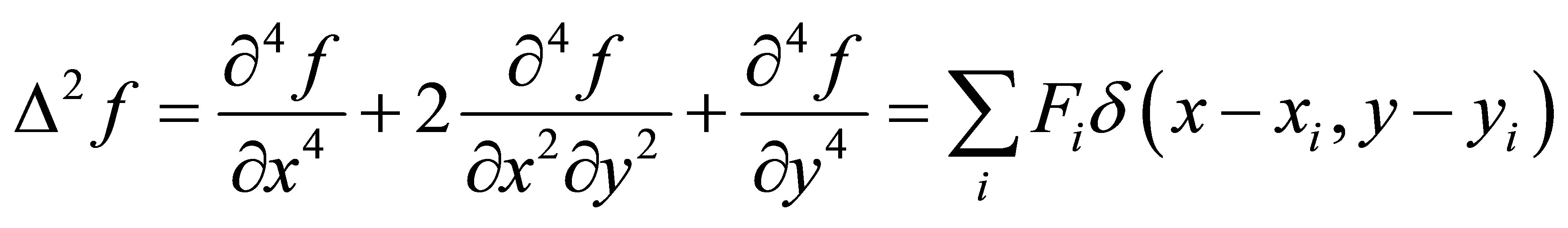
Another option is to use a higher-order harmonic differential equation. The pioneer in this approach was Briggs [10], who used the biharmonic equation
 (2)
(2)
to interpolate gravity and aeromagnetic fields but was limited to regular grids and rectangular, simply-connected regions. The equation is derived by minimizing total domain-integrated squared curvature,  , where
 is the domain on which f is defined.
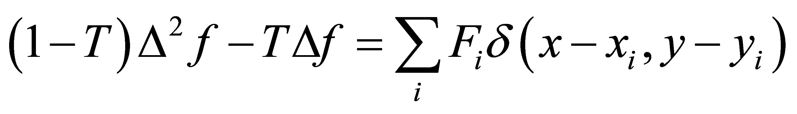
Smith and Wessel [11] further extend Briggs’ work by applying a linear combination of a biharmonic operator and Laplace’s operator:
 (3)
(3)
where T is a tension parameter. Their applications were also restricted to regular grids and rectangular, simplyconnected regions. Equation (3), which we call minimum curvature with tension (MCT), can be thought of as the analog of a thin elastic plate, bent to fit the data points with a tension applied at the boundary. Tension helps to reduce the problem of overshooting.
Higher order harmonic interpolation functions such as  and
and  are also widely applied in graphic processing [12], but their use rarely has been reported in hydrographic and oceanographic applications. We include them here for completeness.
In this paper, we present a new, generalized interpolation method by solving a partial differential equation (PDE) with a linear combination of different orders of harmonic operators (the 1st, 2nd, 3rd and 4th) on an unstructured, triangular-element grid. Our approach has three main advantages over previous solution methods. First, the use of multiple orders of differentials allows for more possible harmonic functions to be incorporated into the solution. With proper parameter selection, we can eliminate the apparent flaw in the occurrence of singularities at the data points when using Laplace’s equation alone. Second, the use of unstructured grids to represent coastal water avoids issues related to interpolation over intervening land features, the necessity of over-water distance calculations, and the problem of multiple connected regions. The third is the streamlining of the multiple-order harmonic PDE interpolation into one simple implementation and solving the equation implicitly without the need for iterations. We note that this approach incorporates the (regular grid) equations of Hess [7], Briggs [10], Smith and Wessel [11], and Botsch and Kobbelt [12] through parameter selection.
We explore the application of the multiple-order harmonic equation to oceanographic properties, namely tidal fields. The outline of the paper is as follows: first, we introduce the mathematics of the governing equations, then we give accounts of the numerical method for the solution, the quantitative measure of error, and the jackknife method of testing. After that, we present four cases of applications: an idealized function in a square domain; Kelvin wave reflection in a semi-infinite rotating channel; M2, S2, K1 and O1 tidal constituents in the Bohai Sea; and the M2 tidal constituent amplitude and phase in Chesapeake Bay. Finally, we offer conclusions based on the applications of the generalized multiple-order harmonic equation interpolation method.
2. Methods
2.1. Governing Equation and Boundary Conditions
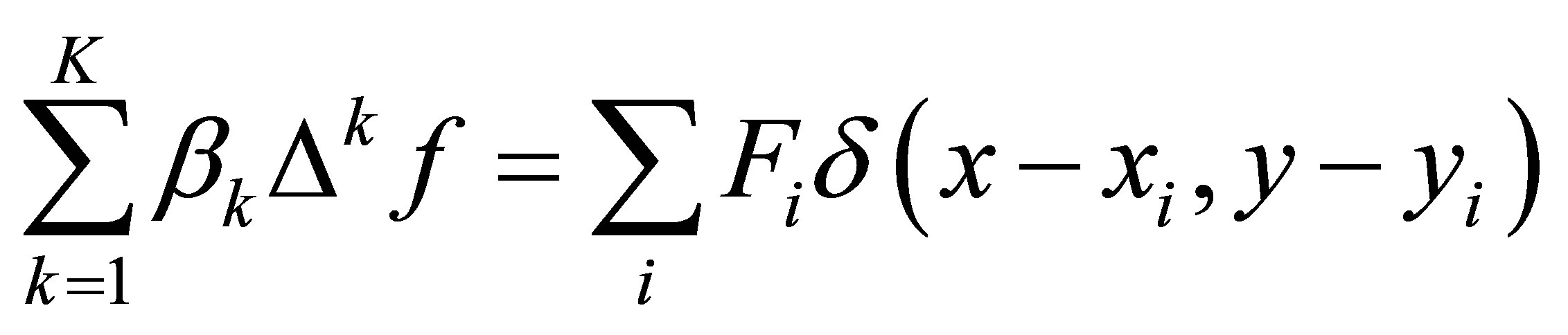
The generalized governing equation for spatial interpolation, which incorporates multiple orders of harmonics, is
 (4)
(4)
where  (k = 1, 2, 3,∙∙∙, K) is the coefficient of the kth order harmonic operator, and with the constraint
 .
.
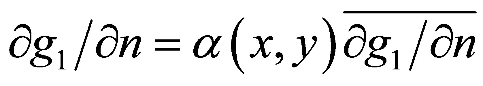
We note that, with appropriate selection of coefficients β, this equation includes Laplace’s equation (Equation (1)), minimum curvature (Equation (2)), and MCT (Equation (3)). Boundary conditions are specified as:
 (5a)
(5a)
 (5b)
(5b)
where  is the normal derivative,
  is an adjustable dimensionless parameter and
  is the spatial average of the normal derivative in a small region adjacent to the boundary. Equation (5a) allows some flexibility in simulating tidal properties, and has been used successfully in computing tidal constituent distributions in Galveston Bay and San Francisco Bay [8].
The left hand side of Equation (4) is a linear combination of different order harmonic operators. By using different combinations of  (k = 1, 2, 3,∙∙∙, K), the solution of Equation (4) provides a class of interpolation methods (Table 1). In our applications, we avoid any order of harmonic operator higher than 4 due to the high computational cost, high computer memory requirements, and the natural tendency towards overshooting or oscillation, which can be especially pronounced in a domain interior in the case of interpolating from boundary data without constraints from internal data points.
Equation (5a) can have different physical explanations, depending on the order and the value of α. For Laplace’s equation, in analogy to a stretched membrane,  corresponds to a zero slope at the boundary, and
  to a constant, non-zero slope at the boundary. For 2nd order or MCT, the equation describes an elastic thin plate. In this case,
  forces the solution to flatten at the edge and
  corresponds to a free-edge condition without bending stress. In general, the α value indicates the degree of balance between the 1st and 2nd normal derivative at the boundary, and it provides a tool to adjust the boundary condition and internal field. In our current application, we take
 , which has been shown to yield realistic solutions to tidal constituent distributions [7].
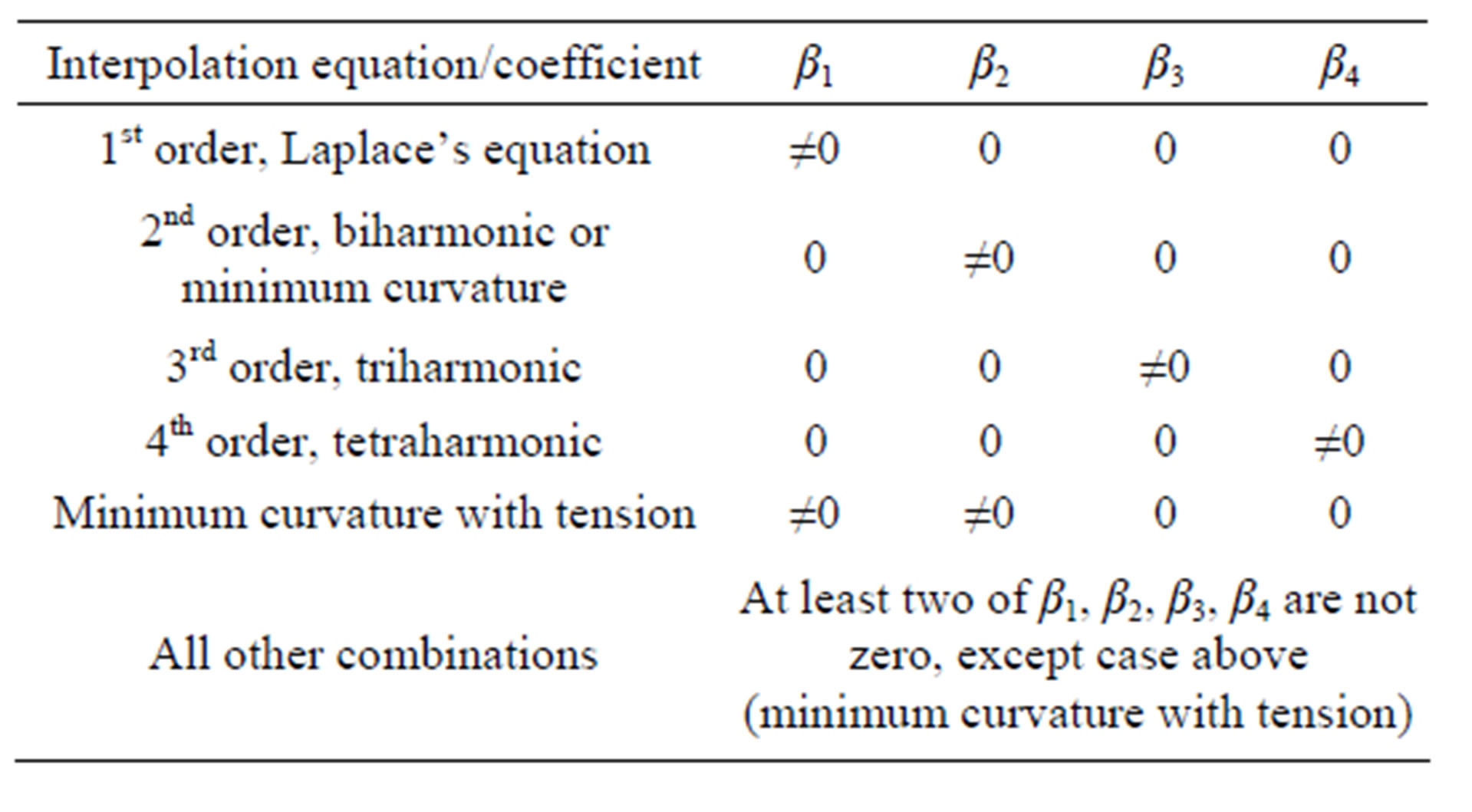
Table 1. Possible combinations of coefficients for different order harmonic operator up to 4th order. Only 1st, 2nd, 3rd, and 4th order harmonic equations and minimum curvature with tension method are explored in this paper. (note: the names of interpolation are interchangeable, as shown in the table. For example, 1st order interpolation will be the same as Laplace’s equation interpolation.)
In addition, many of the equations represented by the different combinations listed in Table 1 can be derived directly from optimization of an energy function through variational calculus [12,13]. For example, for k = 1, Laplace’s equation describes a surface which minimizes the area. For k = 2, a surface that minimizes the curvature is represented, and k = 3 represents a surface that minimizes the variation of linearized curvature. In the onedimensional case, the 1st, 2nd, 3rd, and 4th order harmonic interpolation equations represent piecewise linear, cubic, quintic, and septic polynomial interpolation, respectively.
As will be shown in the next section, the PDE (Equations (4), (5)) can be readily solved using mixed finite element methods with linear triangular elements.
2.2. Mixed Finite Element Method
Laplace’s and Poisson’s equations can be readily solved using a standard finite element method with linear triangular elements [14]. To directly solve a higher order harmonic equation, we employ a mixed finite element method [15-17] to transform Equation (4) into a 1st order linear Poisson’s equation system. First, we assume
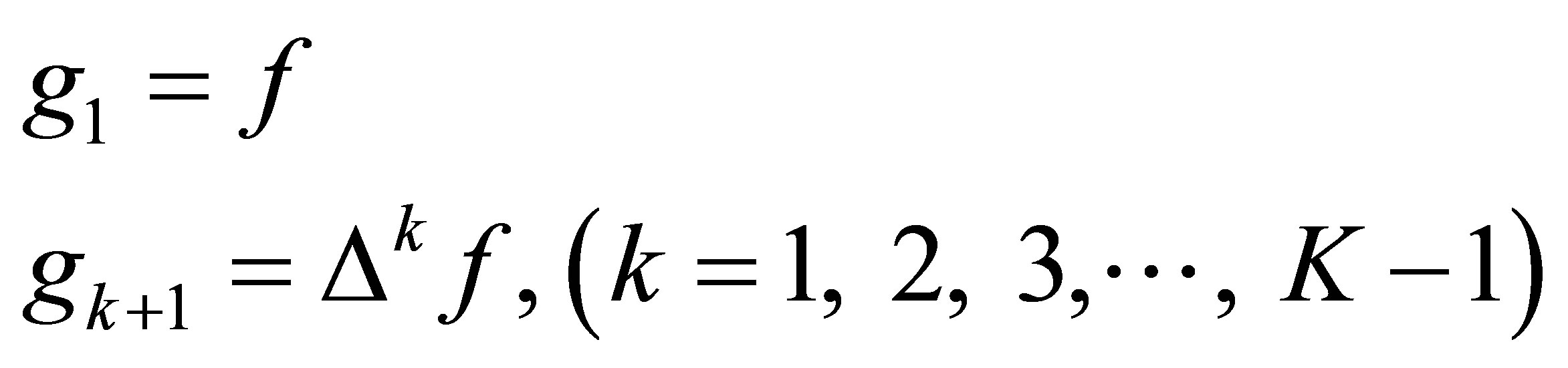 .
.
We then transform the high order linear harmonic Equation (4) into a low order linear PDE system,
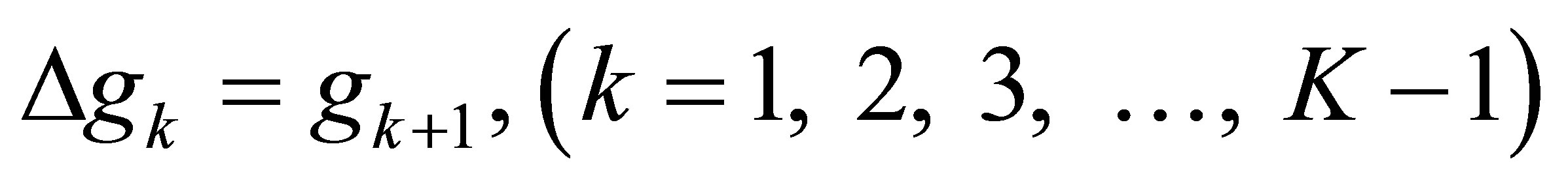 (6a)
(6a)
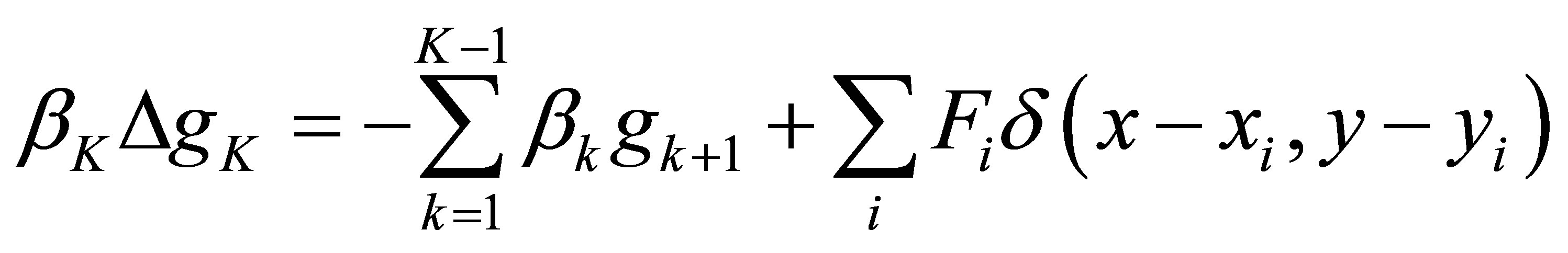 (6b)
(6b)
with the boundary conditions,
 (7a)
(7a)
 (7b)
(7b)
Equation (6b) is a screened Poisson equation. Applying the mixed finite element method to the above mixed PDE system, i.e., Equation (6) with boundary conditions Equation (7), and using a discrete Laplace operator [18, 19], we have a linear system . Here A is a (K × n) × (K × n) sparse matrix for a linear triangular mesh with n nodes. B is a (K × n) column vector.
  is a (K × n) column vector, where Gk (k = 1, 2, 3,∙∙∙, K) is a (1 × n) column vector representing the value of gk (k = 1, 2, 3,∙∙∙, K) at the unstructured triangular mesh nodes. This sparse linear equation AG = B is solvable by straightforward array arithmetic (we used the MATLAB© built-in linear system function). The equation not only solves the interpolation field, but also produces the kth (k = 1, 2, 3,∙∙∙, K − 1) order Laplacian field as a byproduct. The method can also be used for solving the Poisson equation, the Helmholtz equation, and the bi-Helmholtz equation with the addition of appropriate terms to Equation (4).
2.3. Experiments, Error Estimation and the Jackknife Method
To test the generalized multiple-order harmonic spatial interpolation method, we use two different types of data sets. The first type of data set has a known reference field such as an array of observations or an analytic solution. The second type of data set does not have a known reference field, as only the values at a limited number of locations are known. Each type of data set requires a unique experimental approach.
2.3.1. Experiments with a Known Reference Field
Assuming there is a two-dimensional distributed reference data set A containing N points, we randomly subsample A to create a data set B, a subset of A with M points, where . The spatial interpolation method uses B to create an interpolated field C, which has the same size as A and contains values at all locations in the domain. The number of points selected, M, starts at a small value (for example, we use 5), then increases gradually by adding 5 randomly selected points to the previously selected points. The points are selected from the entire domain. Every time 5 additional points are added, interpolation is performed to create a new field C, and the associated maximum absolute error (MAXE), mean absolute error (MAE), and root mean square error (RMSE) are calculated by comparing the interpolated field C with the reference field A. This experiment is designed to quantify the performance of different methods under different data density scenarios.
Since a tidal property is known primarily at locations along the coastal boundary of the ocean domain, we also conduct one parallel experiment with a realistic constraint: select subset B from boundary points only, again starting with 5 randomly-selected boundary points, then adding another 5 boundary points, and so on. The error statistics are calculated with this data series in the same way as for the random selection from all points.
2.3.2. Experiments with an Unknown Reference Field
In many coastal applications, there is no known background reference field, and only scattered station data located mostly along the land-sea boundary are available. Because of a limited number of stations, subsampling may encounter the problem of small total sample size. To reduce the uncertainty due to sample size, we will fix the subsample size and repeat the subsampling for any possible combination. In our application, the delete-1 jackknife method will be used [20]. Specifically, a subsample size of N − 1 out of a total of N samples will be used, and a total of N repeat samplings will be performed by removing one station at a time. At the end we have N error values, one at each station, and the same MAXE, MAE, and RMSE will be calculated. This experiment is designed to quantify the performance of different methods using limited data points at fixed locations without a known reference field.
3. Applications
The performance of the new interpolation method using the high order harmonic PDE is evaluated in four test cases, each with different numbers and distributions of data points and varying complexity of the domain. In each case we first tested pure 1st, 2nd, 3rd and 4th order interpolation. If 3rd and 4th order interpolation is not as good (i.e., has higher error measures) as both 1st and 2nd order interpolation, a few MCT cases are then tested, and the 3rd and 4th order results are not presented. Usually we start by testing the use of all internal and boundary data points, then proceed to testing the use of boundary points only. For the cases in which an analytic solution is known, we test the solution using various harmonics with progressively larger numbers of data points.
3.1. Analytic Function
Here we apply the PDE to an idealized square basin with a known analytic function describing the distribution. Since the reference field is a known analytic function, we may compare the interpolated solution and reference field at any desired point, especially at randomly-selected internal points. The analytic function, Peaks, included in the MATLAB© software, takes the form of:
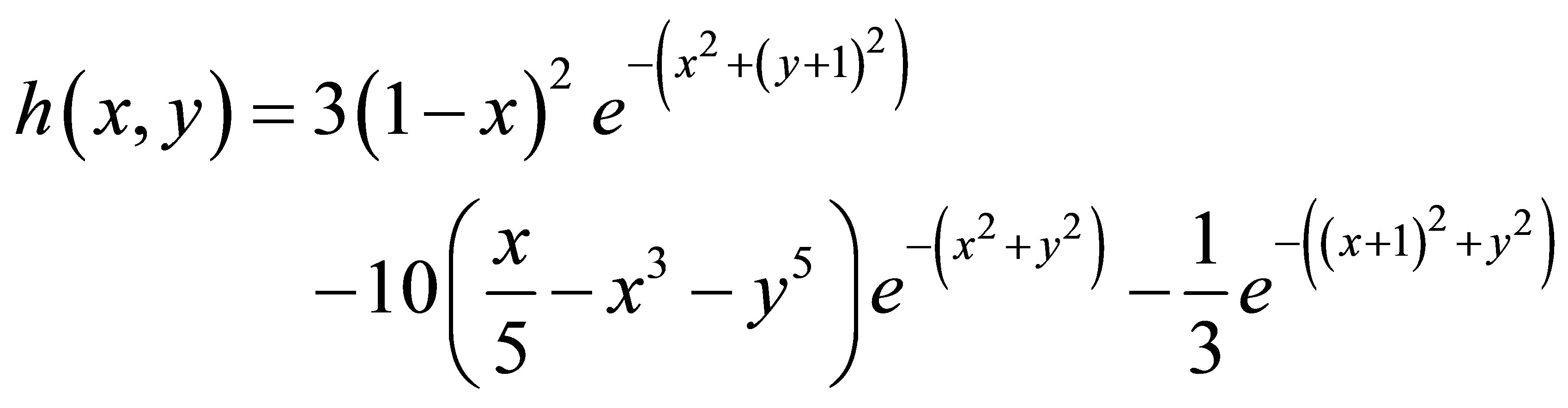 (8)
(8)
Peaks is a combination of three two-dimensional Gaussian functions, each multiplied by a polynomial function, which ensures that the function  approaches zero at locations far from the origin (in our idealized basin, x and y each varies between −3 and 3). The function ranges in value from a minimum of −6 to a maximum of 8. In our experiments, we represent the square basin with an unstructured grid mesh having 161 equally-spaced nodes in the xand y-direction. The reference field was generated by evaluating Equation (8) at the nodes of the mesh.
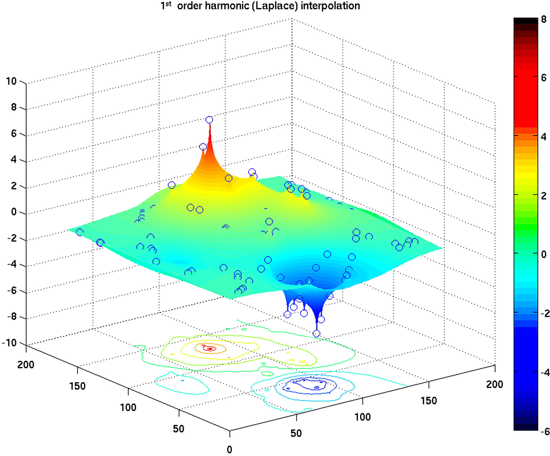
A flaw in the Laplace’s equation solution is very obvious from a plot of the test with 90 random data points, in which singularities occur at the data points (Figure 1(a)), while the higher order harmonic interpolation generates a very smooth surface (Figure 1(b)). The surface contour plots (Figure 2) indicate that the pure 3rd order
 (a)
(a)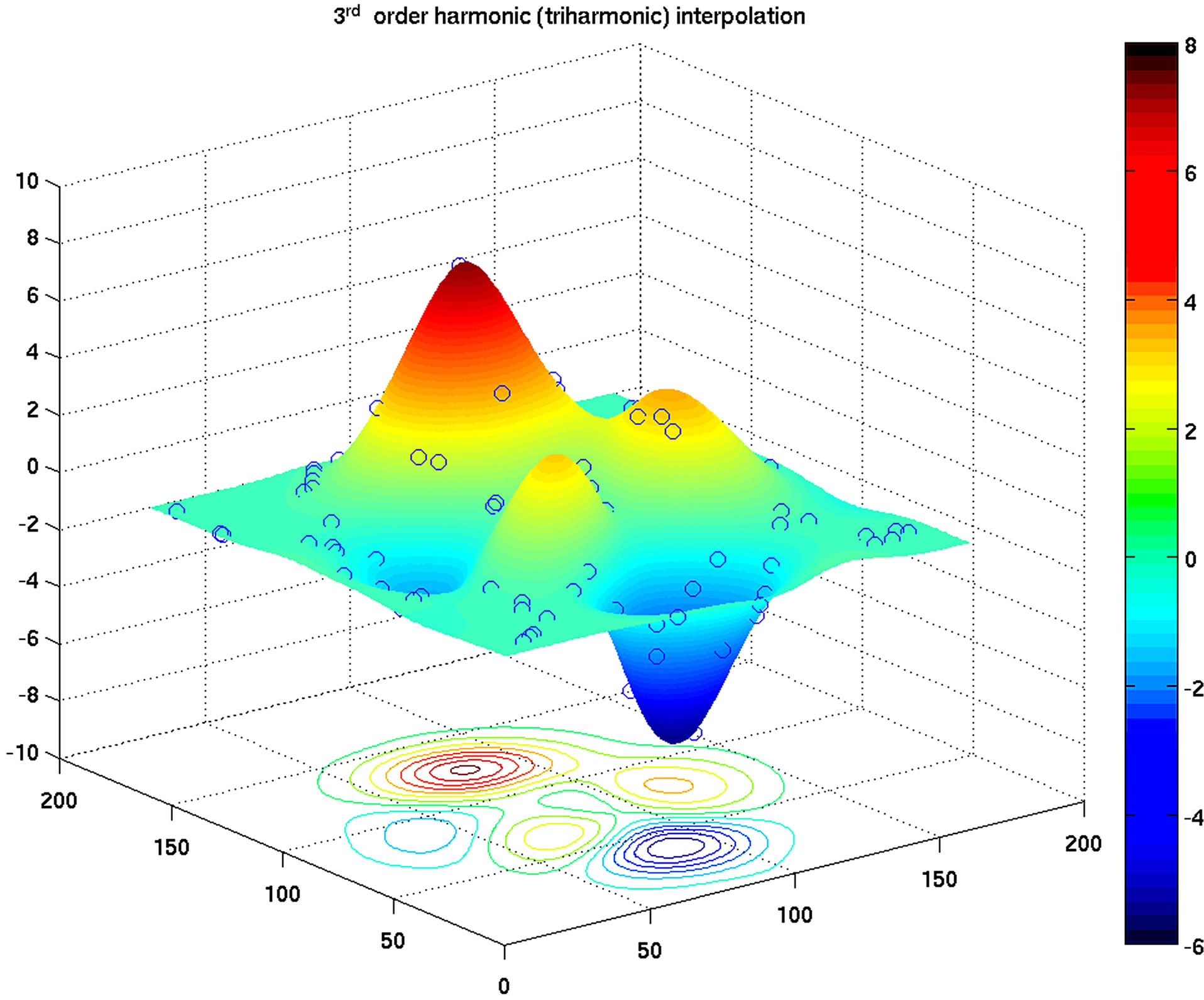 (b)
(b)
Figure 1. Idealized basin and the Peaks function (Equation (8)). (a) Laplace’s equation interpolation with 90 random data points (blue circles). (b) Triharmonic equation interpolation with same data points. Numbers along the axes refer to grid points in the 161 × 161 array.
harmonic interpolation gives the best results, compared to either the 1st or 2nd order interpolation with 90 random data points (this conclusion is also supported by the plots in Figures 3a-c). The MAE for Laplace’s interpolation decreases steadily with an increase in the number of data points. At low data point numbers (M < 25), Laplace’s interpolation performs better than all of the higher order harmonic interpolations. But at the same time, at low data point numbers, the overall error is relatively high, i.e., on the same order of magnitude as the interpolated values. With an increase in the number of data points, the higher order harmonic interpolations, especially the 3rd and 4th order harmonic equations, improve much faster than the Laplace’s interpolation. When the number of
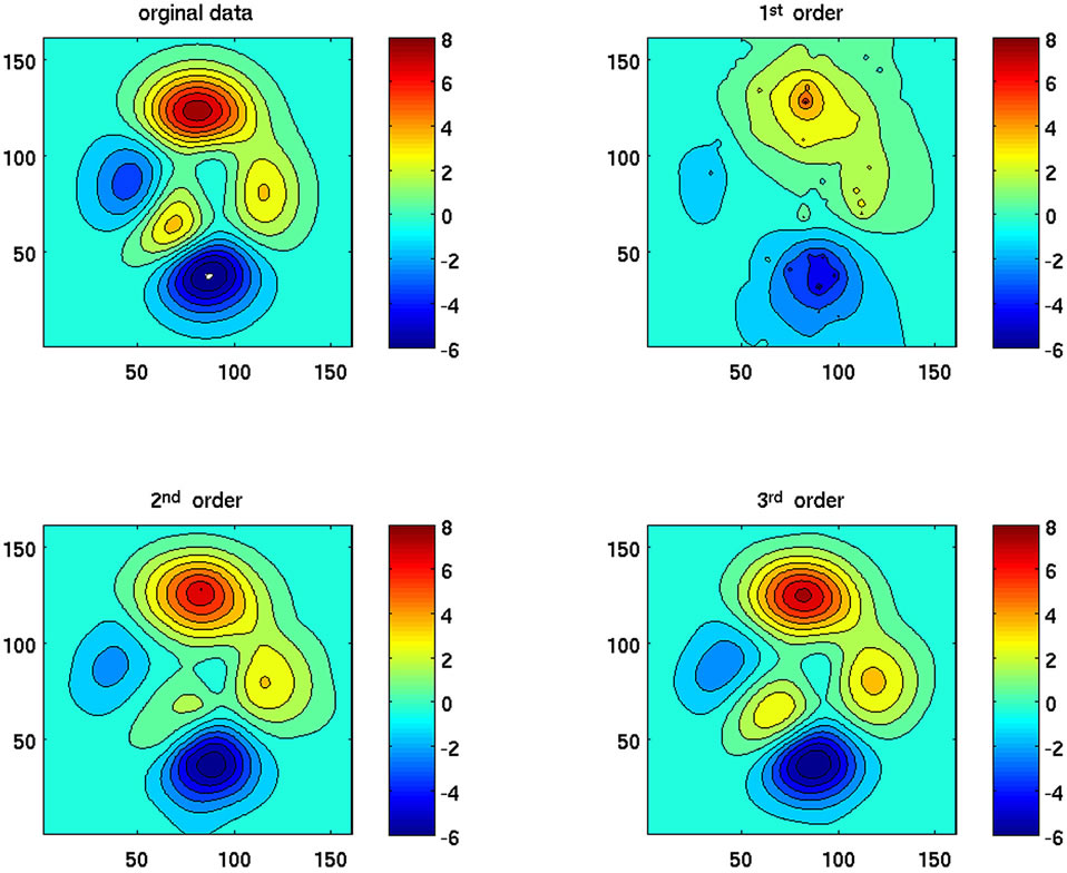
Figure 2. Idealized basin and the Peaks function (Equation (8)). Inter-comparison of two-dimensional contour plots between the original data and the 1st, 2nd, and 3rd order interpolation with 90 random data points. Numbers along the axes refer to grid points in the 161 × 161 array.
observed points increases to 100, the 4th order outperforms the 3rd order. The trends from all three error measures are similar in that they decrease with increasing number of data points, although the errors decrease faster with the higher order. As for the use of boundary points only, we note that since the values along the boundary are all very close to zero, interpolation using only boundary points will not yield much useful information about the interior of the basin. We therefore do not present any results from boundary only data.
In general, high order interpolation gives a smooth solution with a continuous derivative within the domain, including at the data points. For all interpolation methods, errors decrease when more data points are used. The higher-order PDEs outperform lower-order PDEs, except when the number of data points is small (M < 25).
3.2. The Taylor Problem
The original Taylor problem, which was first presented and solved analytically by Taylor [21], is the Kelvin wave reflection in a semi-infinite rotating channel without friction. In our experiments, to be consistent with Taylor [21], we simulated flow in a channel that is 500.4 km wide (north to south), 74 m deep, and 1000 km long, east to west (Figure 4). The Coriolis coefficient is 0.000119 s−1 (corresponding to latitude 54.46˚N) and the period of oscillation was set to 12.4 hours to approximate the M2 period. This example was selected because it has an analytic solution for tidal amplitude and phase distribution, thus providing a reference field, and unlike the previous case it has non-zero boundary values. The dominant feature in the analytic solution is a chain of
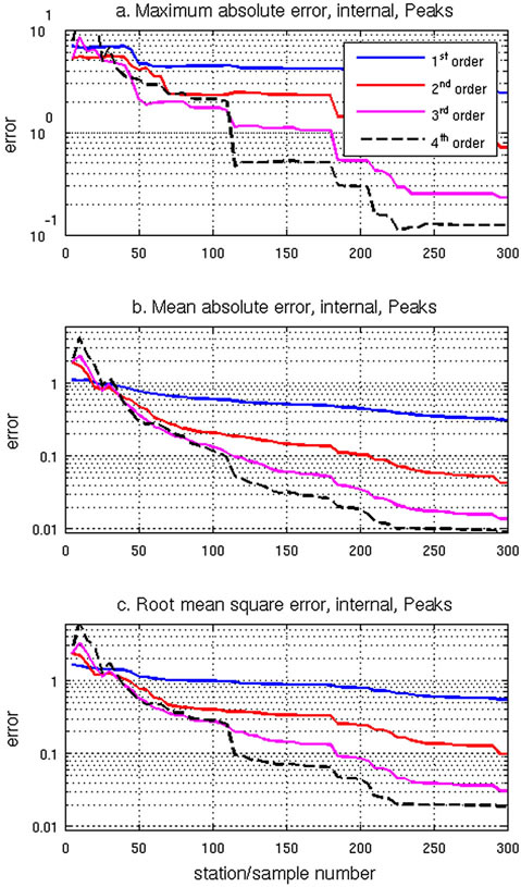
Figure 3. For the idealized basin, the maximum absolute error (MAXE), mean absolute error (MAE), and root mean square error (RMSE) of 4 different order harmonic equation interpolations, and their variation with the increase of internal data points of Peaks: a) MAXE; b) MAE; c) RMSE.
amphidromes along the center line of the channel. Rienecker and Teubner [22] introduced friction (with a coefficient of 0.00005 s−1), and with friction the amphidromes shift laterally from the center line of the channel to the right side of the channel if facing the inbound wave (Figure 4a). There are two amphidromes within the first 1000 km of the channel. The first amphidrome is close to the center line. Further away from the closed western end, the wave is attenuated and the second amphidrome is closer to the southern boundary. Depending on the bottom friction, the amphidrome may be degenerated, and the center may move inland, producing a virtual amphidrome.
To create the interpolation we use an unstructured triangular grid having a uniform 5 km resolution with a
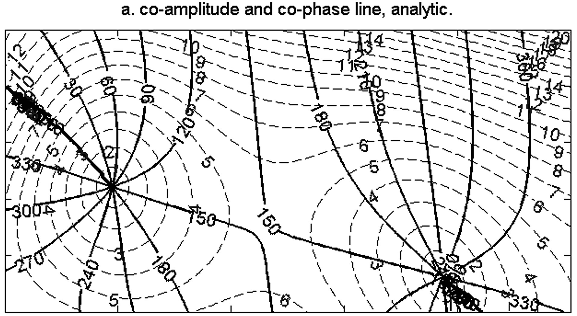
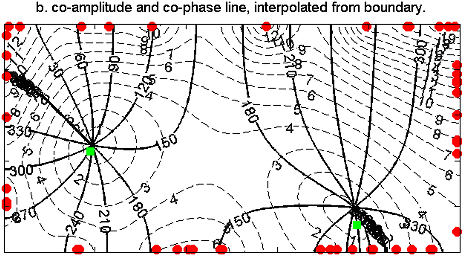
Figure 4. Taylor basin solution (the M2 tide in a semi-infinite rotating channel). The coamplitude (dashed) and cophase (solid) lines for a) analytic results [22] and b) interpolated from 40 random boundary points using 2nd order interpolation. The green dots are the amphidrome locations from analytic solution.
total number of 20,301 nodes. A tidal constituent consists of amplitude A and phase φ, which can be expressed as a complex number,  , where R is the real part and E is the imaginary part of the number. We interpolate R and E separately, and after interpolation, we reverse the calculation,
  , and
, and . This complex number interpolation is also used for the interpolation of the M2 tidal constituent in the following Bohai Sea and Chesapeake Bay cases.
Two tests were conducted for the Taylor case, one interpolated from random internal and boundary data points and the other from only random boundary points. For both tests, along with the usual statistics, another statistic was computed: the average distance between amphidromes in the reference field (here the analytic solution) and corresponding amphidromes in the interpolated field.
In the internal points case, locations of the amphidromes are able to converge quickly (M > 50) to the analytic positions (Figure 5d). For both amplitude and phase, the 2nd order interpolation dramatically reduces the error in MAXE, MAE, RMSE, and the distance between the amphridromes (Figure 5) in comparison with the 1st order interpolation. The 1st order interpolation error is about 10 times that of the 2nd order interpolation error in all three measures. The 3rd order interpolation is consistently better than the 2nd order, but only by a small margin (i.e., only a few percent). The 4th order is comparable to the 3rd order, or slightly better, especially for large data numbers (M > 600). However, the 4th order interpolation performance can deteriorate (most likely from overshooting) as demonstrated by a sudden increase in RMSE at M = 250 (Figure 5f), although it is still better than the 1st order and performance improves with further increase of data points (M > 600).
In the boundary points only case, besides the pure 1st and 2nd order interpolations, we tested three interpolations using MCT, with pairs of coefficients  = (0.5, 1), (0.2, 1), and (0.1, 1). We do not present results for the 3rd and 4th order for the boundary case because we found that the 2nd order interpolation consistently outperforms both the 3rd and 4th order in all error measures. The errors decrease with increasing number of boundary data points for both amplitude and phase for the 1st order and the three MCT cases. The order of their performance in decreasing magnitude of error corresponds to
  values of (1, 0), (0.5, 1), (0.2, 1), and (0.1, 1). By contrast, the pure 2nd order performance is different for amplitude and phase. For amplitude, there is relatively high accuracy at a low data point number (M < 35), but performance deteriorates very quickly with the increase of boundary point number, and the 2nd order interpolation is outperformed by all other methods (Figures 6a-c). For phase, the 2nd order performs the best (Figures 6e and f). With the increase of boundary data points, the phase and amphidrome position improve quickly initially, and after a certain number, the improvement from the additional points levels off. That is reflected in the flat line from M = 150 points and beyond (Figures 6d-f). The interpolated amphidrome is further offshore as compared with the analytic results (Figure 6b), especially for the rightmost amphidrome. Unlike the internal point case, information from the boundary, no matter how detailed, cannot indefinitely improve the results or provide all necessary information for the interior, even when there is still a room to improve.
Thus we can conclude that for the internal points case
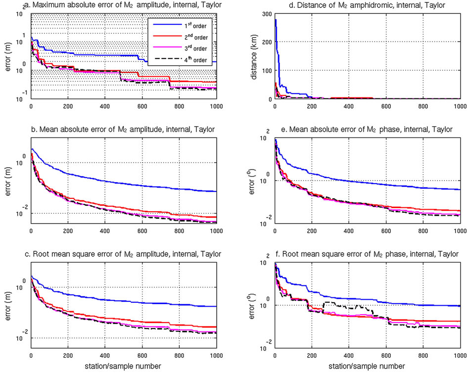
Figure 5. For the Taylor basin (the M2 tide in a semi-infinite rotating channel), the MAXE, MAE, RMSE and amphidrome distance of four different order harmonic equation interpolations, and their variation with incremental internal data points. a) MAXE, amplitude; b) MAE, amplitude; c) RMSE, amplitude; d) amphidrome distance; e) MAE, phase; f) RMSE, phase.
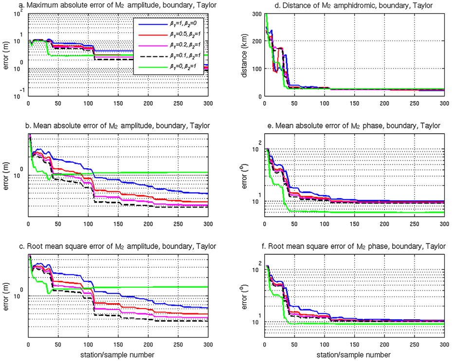
Figure 6. For the Taylor basin, the MAXE, MAE, RMSE and amphidrome distance of five different interpolations, and their variation with incremental boundary data points. M2 tide in a semi-infinite rotating channel. a) MAXE, amplitude; b) MAE, amplitude; c) RMSE, amplitude; d) amphidrome distance; e) MAE, phase; f) RMSE, phase.
in a semi-infinite rotating channel, the 2nd order interpolation provides a solution that dramatically reduces the error to 10% of that for the 1st order interpolation of both M2 amplitude and phase. The use of the 3rd and 4th order terms subsequently further improves the solution, but with a much smaller margin. For the boundary points only case, the phase is best simulated using the 2nd order or 3rd order solution (3rd order results are not presented). For amplitude, though, MCT gives better solutions. Overall, of the limited pairs of coefficients tested, the solution for  = (0.1, 1.0) provided the best results for both amplitude and phase. Finally, in the absence of internal data, an increase in the number of boundary data points does not improve the accuracy of the position of the amphidrome after a certain number of data points (M > 150).
3.3. Tides in the Bohai Sea
The Bohai Sea is a semi-enclosed embayment on the coast of China in the northwest Pacific Ocean, and its tidal system has been well documented from observations and hydrodynamic model simulations [23-25]. The test data set for this case consists of M2, K1, S2, and O1 tidal constituents from 31 observed tidal stations in the Bohai Sea [23], of which 29 are near the coast, and two are from islands in the mouth of the Bohai Sea. To carry out the interpolations, we generated an unstructured grid with 101,217 nodes, having on average a 1 km resolution.
We tested five pairs of  to estimate the performance of different interpolation schemes of the complex solution using the jackknife method (Table 2). For all tidal constituents and for both amplitude and phase, except for the K1 phase, there are more than three combinations of
  that perform better than the 1st order. The 2nd order is better than the 1st order in all amplitudes of the four tidal constituents, and better than the 1st order in MAE, and RMSE for the phase of all tidal constituents. The 2nd order interpolation has worse phase MAXE for the K1, S2, and O1 constituents. For the K1
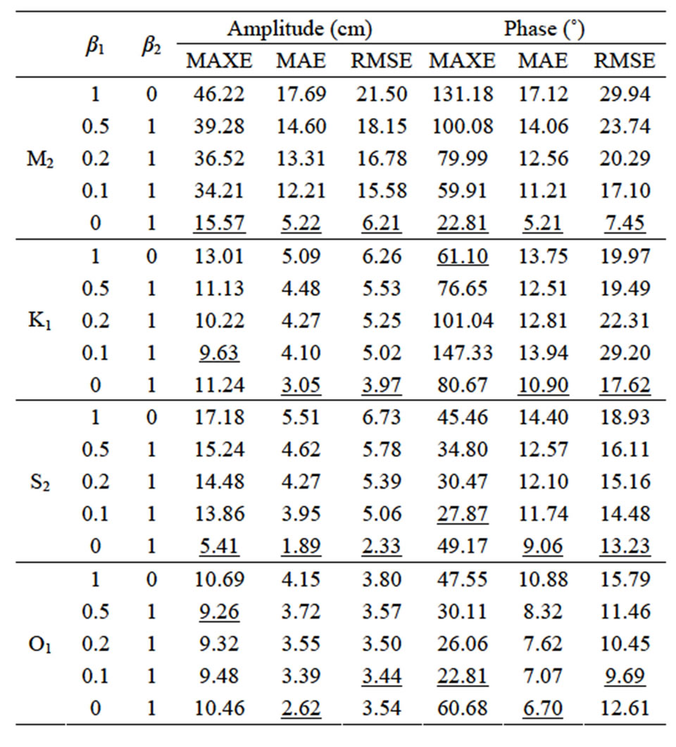
Table 2. Results for the Bohai Sea. MAXE, MAE, and RMSE of amplitude and phase for the M2, S2, K1 and O1 tidal constituents for different interpolation methods using 31 data stations. Underlined values are the best results for five pairs of (β1, β2) in a single error measure.
phase, the 1st order MAXE is the smallest of all methods. That is the only case that there is no better alternative  than the 1st order in all three measures. The 2nd order gives the best results in K1 phase, as measured by the MAE and RMSE (Table 2).
The dominant feature of the results using 2nd order harmonic interpolation is the amphidromic system (Figure 7). For example, the M2 tide system indicates an amphidrome in the north, and possibly a degenerated amphidrome in the west. The location of the amphidromes for all constituents is very close to the position estimated by Fang et al. [24] from altimetry and observed station data (Table 3). As in the Taylor boundary case, the interpolated position of the semi-diurnal amphidrome is slightly more offshore than the estimation, while the diurnal amphidrome’s position is almost identical.
In general, both the pure 2nd order  = (0, 1) and the MCT
  = (0.1, 1.0) give the best results for all four tidal constituents.
3.4. Tides in the Chesapeake Bay
The Chesapeake Bay, on the U.S. East Coast, is representative of an embayment with a long, complex coast whose shoreline length is extremely large compared with its area. In addition, most data locations are situated along the shore and are thus not representative of internal conditions. In this case, the interpolation of the M2 tide,
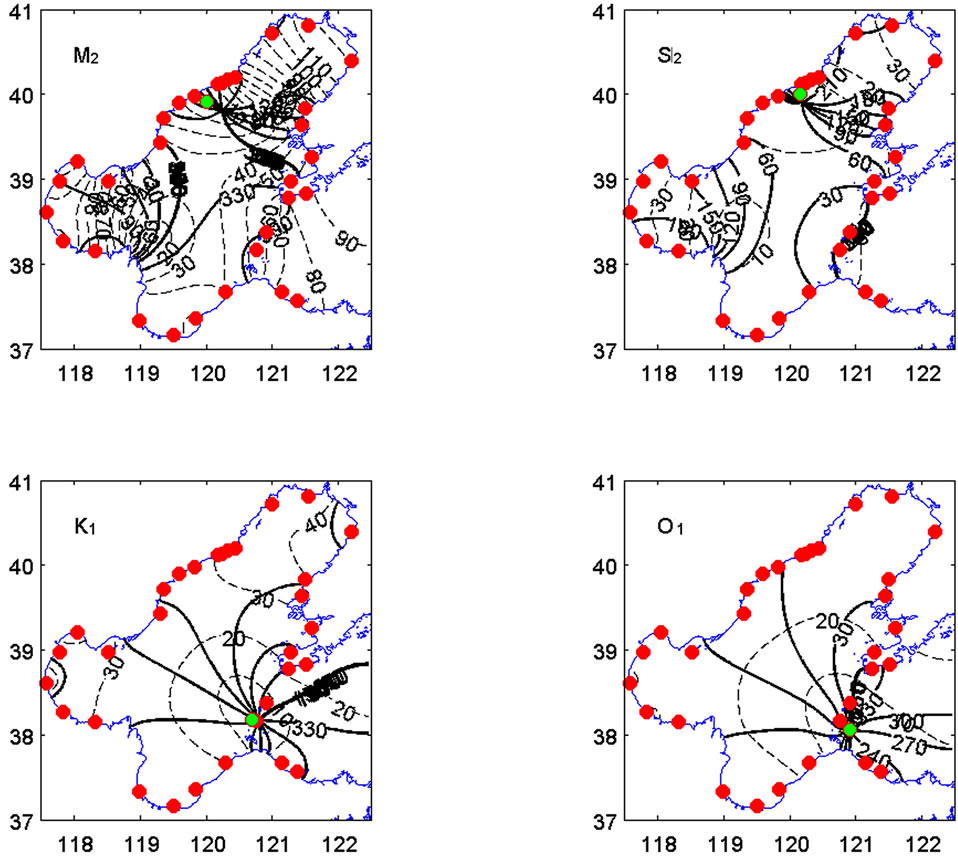
Figure 7. Bohai Sea M2, S2, K1, and O1 cophase lines in degrees (solid line) and coamplitude lines in meters (dashed line). Also displayed are 29 data stations along the coast, and two island stations near the entrance (red dots). The green dots are the amphidrome locations from Fang et al. [24].
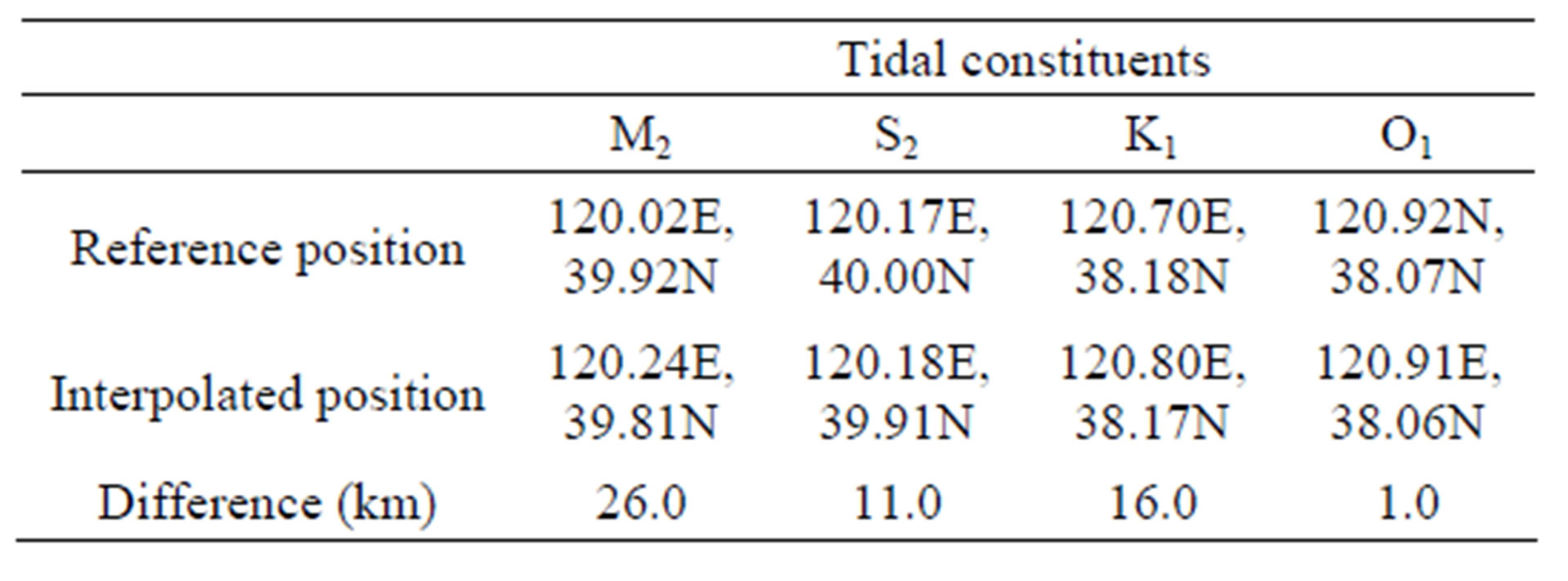
Table 3. For the Bohai Sea tidal constituents, the location of amphidromes from the Fang et al. [24] model (reference position), our interpolation results, and the approximate spatial difference between the two. Results are for 2nd order harmonic interpolation only.
from which the coamplitude and cophase lines are extracted, will be performed and compared using only the 1st order, 2nd order, and MCT interpolation. The unstructured mesh grid we used has 318,860 nodes, and a spatial resolution varying between 0.02 and 20 km [26].
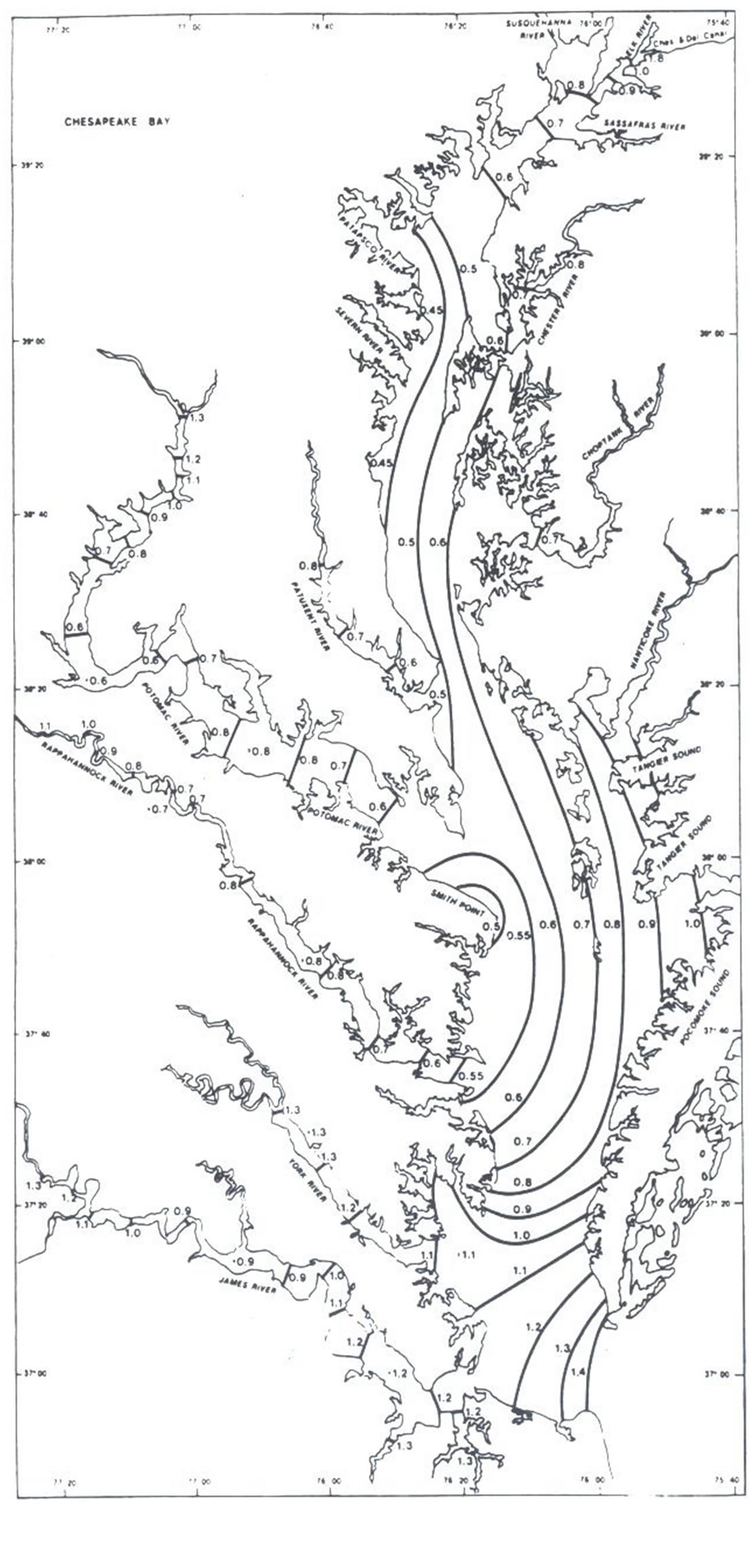
For comparison purposes, the coamplitude (Figure 8a) and cophase (Figure 9a) lines for the Chesapeake Bay are hand-drawn contour plots from Browne and Fisher [27], using data from 121 present and historical tide stations. There are two features in the tidal amplitude field that are the most apparent. First, as is the situation in the Taylor case, the amplitude is usually higher in the Bay’s east side, or the left side when facing the incoming tide wave. This is due to the existence of a virtual amphidrome (i.e., an amphidrome whose center is located on land) just south of latitude 38˚N [27]. Second, the tidal amplitude can either increase or decrease in the direction of wave propagation, while the tidal phase is al-
 (a)
(a)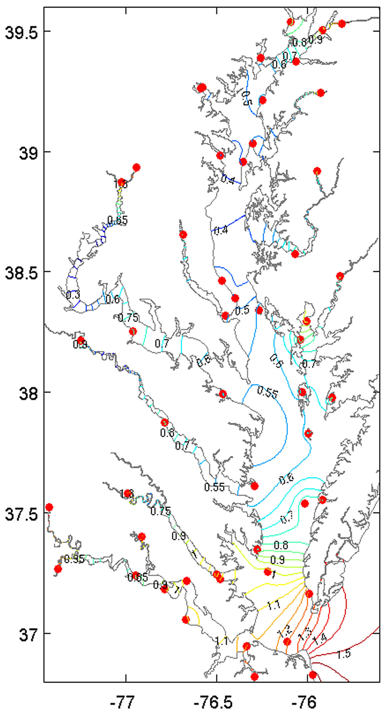 (b)
(b)
Figure 8. Chesapeake Bay M2 coamplitude lines in feet. (a) Hand drawing from historical data (Reproduced from Browne and Fisher [27]). (b) Interpolated field using generalized minimum curvature interpolation (β1 = 0.5, β2 = 1) and 50 tide stations (red dots).
 (a)
(a) (b)
(b)
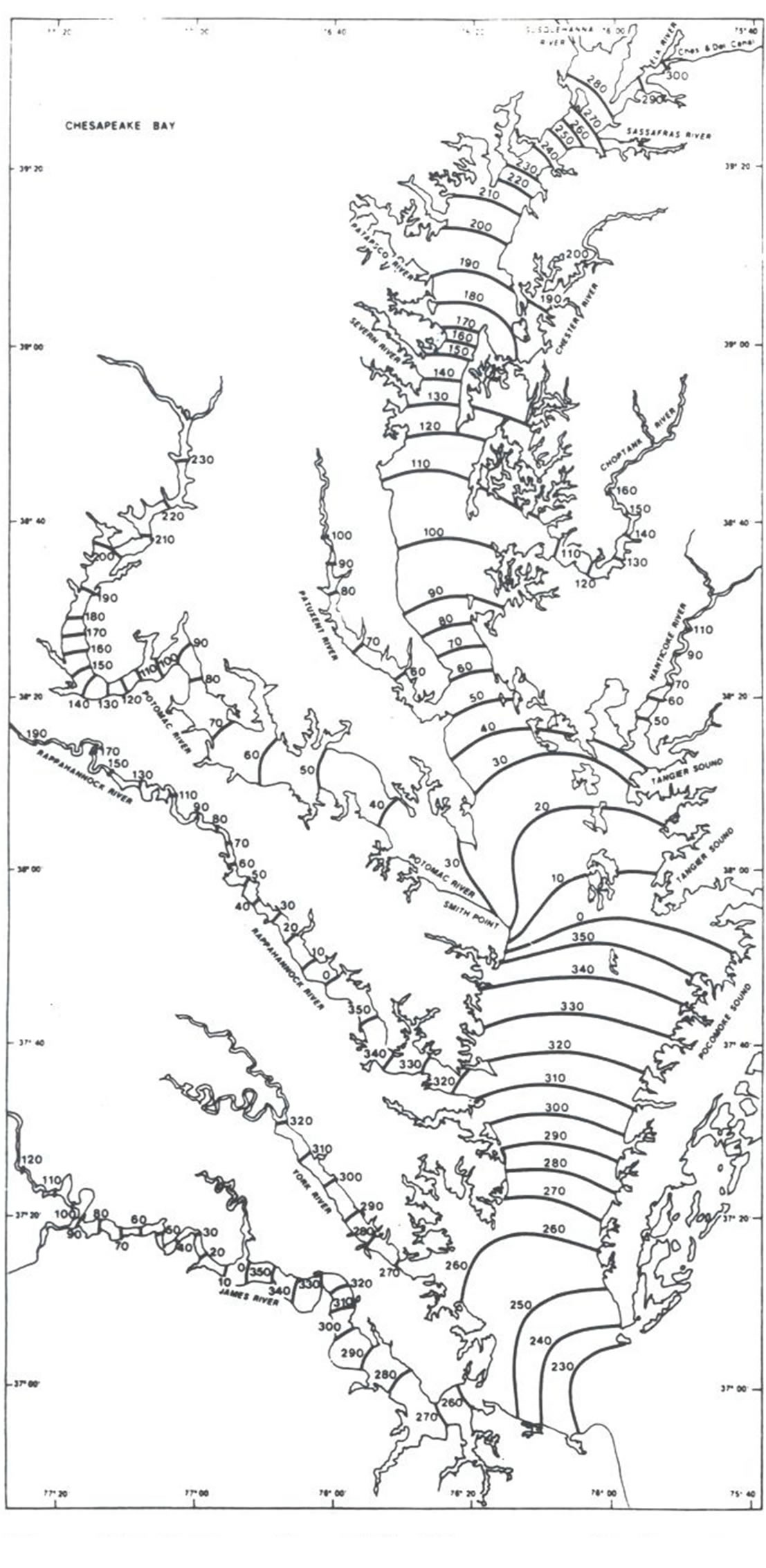
Figure 9. Chesapeake Bay M2 cophase lines in degrees. (a) Hand drawing from historical data (Reproduced from Browne and Fisher [27]). (b) Interpolated field using 2nd order harmonic interpolation (β1 = 0.0, β2 = 1) and 50 tide stations (red dots).
ways monotonically increasing. The behavior of the phase indicates that the tide in the Bay is a progressive wave.
In our Chesapeake Bay application, the M2 tidal constants are obtained from 50 NOS tide stations that had long term tide observations and tidal constituent analysis. The error analysis using jackknifing (Table 4) indicates the results would be the best when using different pairs of β values for amplitude and phase. If we look individually,  = (0.01, 1) is the best for M2 amplitude. However for M2 phase, the 2nd order interpolation is the best.
The resulting interpolated fields of M2 coamplitude and cophase for the optimal pair of  are presented in Figures 8 and 9, respectively. The major features of the amplitude (i.e., the virtual amphidrome) and phase are reproduced. The MAE of the amplitude interpolation is about 5.90 cm. The phase distribution is more regular and monotonic with a MAE of 13.45 degree using the 2nd order interpolation (Figure 9).
4. Summary and Conclusions
In this paper, we developed a PDE containing multiple, high order harmonics for spatial interpolation of tidal properties in the coastal ocean. The equation is solved on an unstructured triangular grid with a mixed finite element method. The use of an unstructured grid allows for the representation of geometrically complex regions, including islands, and eliminates the need for over-water distance calculations or interpolating across land. In its numerical implementation, the method avoids iteration, which may not converge, and instead uses a simple implicit procedure. Four test cases have been examined,
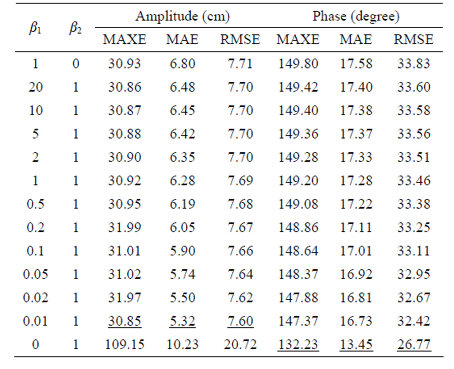
Table 4. Results for the Chesapeake Bay. Comparison of M2 tide amplitude and phase errors using 1st order, MCT and 2nd order interpolation. The results are derived using the jackknife method. Underlined values are the best results of 13 pairs of (β1, β2) in a single error measure.
including an idealized function in a square basin, tidal properties in a semi-infinite rotating channel, tides in the Bohai Sea, and tides in the Chesapeake Bay. The results demonstrate that the multiple-order harmonic interpolation method eliminates the singularities at the observed data points that occur in Laplace’s equation interpolation (Figure 1b). It also reduces the computed error and improves the accuracy and precision of the interpolated field when appropriate values of the adjustable parameter (i.e., the values of β, Table 1). Computationally, the method is comparable in speed to the solution of Laplace’s equation by iteration.
In all our test cases, the optimal combination of coefficients  (k = 1, 2, 3,∙∙∙, K) is highly dependent on the spatial characteristics of the interpolated property, complexity of the boundary, and the number and spatial distribution of the data points. In practice, different combinations of coefficients have to be tested to find an optimal combination. It is advisable to test pure 1st, 2nd, 3rd and 4th order interpolations first. If 3rd and 4th order interpolations do not reduce errors, they should be ignored and then MCT cases should be tested. The optimal combination of coefficients can be determined by evaluating the error measures from these tests.
To interpolate the tidal constituents’ amplitude A and phase φ, it is good practice to separately interpolate the real part R and imaginary part E of the complex number representation, . In our experience, the interpolated R and E fields are usually smoother than amplitude and phase, with maxima and minima at the domain boundary.
Interpolation from boundary data alone can produce good results for tidal properties (Figures 4, 6e and f), but has its limits. No matter how dense the data points are, the missing information from the interior (i.e., offshore) will never be fully recovered from the boundary data alone. This is demonstrated by the persistent error in the distance between amphidromes between the reference field and the interpolated field (Figure 6d), and the flat line of error measures when increasing the number of boundary points (Figures 6a-f).
In practice, tidal amplitude and phase can be interpolated separately, each using different values of β coefficients to achieve an optimal result, as demonstrated in the Taylor basin and the Chesapeake Bay M2 tide cases. For amplitude in those cases, MCT is better than either the 1st order or the 2nd order interpolation alone (Figures 6a-c; Table 4). For phase, the 2nd order interpolation is the best in all three error measures in Chesapeake Bay (Table 4), as well as for M2 phase in the Taylor boundary point case (Figures 6d-6f). The fact that different values of β produce optimal results may be due to differences in the underlying properties of tidal amplitude and tidal phase. In other words, the tidal phase field is much smoother than the tidal amplitude field, and therefore the tidal phase is more suitable for a higher order harmonic interpolation.
In summary, our development of the high order harmonic interpolation provides a full set of options for the user to choose from for their specific application. Besides being a better tool to achieve more accurate interpolation results, there are also many potential benefits. For example, in hydrographic and oceanographic applications, decisions often have to be made on new locations for data collection. Optimizing the installation of data observation stations (or temporary water level stations for storm surge) may be achieved by differentiating multiple potential station sites by their improvement in overall error measures using this interpolation method.
REFERENCES
- I. K. Crain, “Computer Interpolation and Contouring of Two-Dimensional Data: A Review,” Geoexploration, Vol. 8, No. 2, 1970, pp. 71-86. http://dx.doi.org/10.1016/0016-7142(70)90021-9
- D. F. Watson, “Contouring: A Guide to the Analysis and Display of Spatial Data,” Pergamon, Oxford, 1982.
- R. Daley, “Atmospheric Data Analysis,” Cambridge University Press, Cambridge, 1991.
- S. L. Barnes, “A Technique for Maximizing Details in Numerical Weather Map Analysis,” Journal of Applied Meteorology, Vol. 3, No. 4, 1964, pp. 396-409. http://dx.doi.org/10.1175/1520-0450(1964)003<0396:ATFMDI>2.0.CO;2
- J. F. Turner, J. C. Iliffe, M. K. Ziebert, C. Wilson and K. J. Horsburgh, “Interpolation of Tidal Levels in the Coastal Zone for the Creation of a Hydrographic Datum,” Journal of Atmospheric and Oceanic Technology, Vol. 27, No. 3, 2010, pp. 605-613. http://dx.doi.org/10.1175/2009JTECHO645.1
- W. Collier, G. Glang and L. C. Huff, “Managing Tidal Information for Hydrographic Surveys,” Proceeding of the Eleventh Biennial International Symposium of the Hydrographic Society, Special Publication No 40, University of Plymouth, Plymouth, 1999, pp. 5-7.
- K. W. Hess, “Spatial Interpolation of Tidal Data in Irregularly-Shaped Coastal Regions by Numerical Solution of Laplace’s Equation,” Estuarine, Coastal and Shelf Science, Vol. 54, No. 2, 2002, pp. 175-192. http://dx.doi.org/10.1006/ecss.2001.0838
- K. W. Hess, “Water Level Simulation in Bays by Spatial Interpolation of Tidal Constituents, Residual Water Levels, and Datums,” Continental Shelf Research, Vol. 23, No. 5, 2003, pp. 395-414. http://dx.doi.org/10.1016/S0278-4343(03)00005-0
- K. W. Hess, M. Kenny and E. Myers, “Standard Procedures to Develop and Support NOAA’s Vertical Datum Transformation Tool, VDATUM,” NOAA NOS Technical Report, 2012.
- I. C. Briggs, “Machine Contouring Using Minimum Curvature,” Geophysics, Vol. 39, No. 1, 1974, pp. 39-48. http://dx.doi.org/10.1190/1.1440410
- W. H. F. Smith and P. Wessel, “Gridding with Continuous Curvature Splines in Tension,” Geophysics, Vol. 55, No. 3, 1990, pp. 293-305. http://dx.doi.org/10.1190/1.1442837
- M. Botsch and L. Kobbelt, “An Intuitive Framework for Real-Time Freeform Modeling,” ACM Transactions on Graphics (TOG), Vol. 23, No. 3, 2004, pp. 630-634. http://dx.doi.org/10.1145/1015706.1015772
- W. Welch and A. Witkin, “Variational Surface Modeling,” Computer Graphics (Proceedings of ACM SIGGRAPH 92), 1992, pp. 157-166.
- P. G. Ciarlet, “The Finite Element Method for Elliptic Problems,” North Holland, Amsterdam, 1978.
- R. S. Falk, “Approximation of the Biharmonic Equation by a Mixed Finite Element Method,” SIAM Journal on Numerical Analysis, Vol. 15, No. 3, 1978, pp. 556-567. http://dx.doi.org/10.1137/0715036
- F. Brezzi and M. Fortin, “Mixed and Hybrid Finite Element Methods,” Springer-Verlag, New York, 1991.
- X. Cheng, W. Han and H. Huang, “Some Mixed Finite Element Methods for Biharmonic Equation,” Journal of Computational and Applied Mathematics, Vol. 126, No. 1-2, 2000, pp. 91-109. http://dx.doi.org/10.1016/S0377-0427(99)00342-8
- M. Desbrun, M. Meyer, P. Schroder and A. H. Barr, “Implicit Fairing of Irregular Meshes Using Diffusion and Curvature Flow,” Proceeding of ACM SIGGRAPH 99, ACM Press/ACM SIGGRAPH, 1999, pp. 65-72.
- M. Meyer, M. Desbrun, P. Schroder and A. H. Barr, “Discrete Differential Geometry Operators for Triangulated 2- Manifolds,” In: H. C. Gege and K. Polthier, Eds., Visualization and Mathematics III, Springer-Verlag, New York, 2003, pp. 35-57.
- W. J. Emery and R. E. Thomson, “Data Analysis Methods in Physical Oceanography,” Elsevier Science, 2001.
- G. L. Taylor, “Tidal Oscillations in Gulf and Rectangular Basins,” Proceedings of the London Mathematical Society, Vol. 20, 1920, pp. 148-181.
- M. M. Rienecker and M. D. Teubner, “A Note on Frictional Effects in Taylor’s Problem,” Journal of Marine Research, Vol. 38, 1980, pp. 183-191.
- C. Chen, H. Liu and R. C. Beardsley, “An Unstructured, Finite Volume, Three-Dimensional, Primitive Equation Ocean Model: Application to Coastal Ocean and Estuaries,” Journal of Atmospheric and Oceanic Technology, Vol. 20, No. 1, 2003, pp. 159-186. http://dx.doi.org/10.1175/1520-0426(2003)020<0159:AUGFVT>2.0.CO;2
- G. Fang, Y. Wang, Z. Wei, H. H. Choi, X. Wang and J. Wang, “Empirical Cotidal Charts of the Bohai, Yellow, and East China Seas from 10 Years of TOPEX/Poseidon Altimetry,” Journal Geophysical Research, Vol. 109, No. C11, 2004, pp. 1-13. http://dx.doi.org/10.1029/2004JC002484
- J. Wang, Y. Shen and Gao, “Seasonal Circulation and Influence Factors of the Bohai Sea: A Numerical Study Based on Lagrangian Particle Tracking Method,” Ocean Dynamics, Vol. 60, No. 6, 2010, pp. 1581-1596. http://dx.doi.org/10.1007/s10236-010-0346-7
- Z. Yang, E. P. Myers, A. M. Wong and S. A. White, “VDatum for Chesapeake Bay, Delaware Bay, and Adjacent Coastal Water Areas: Tidal Datums and Sea Surface Topography,” NOAA NOS Technical Memorandum NOS CS 15, 2008.
- D. R. Browne and C. W. Fisher, “Tide and Tidal Currents in the Chesapeake Bay,” NOAA Technical Report NOS OMA 3, 1988.
NOTES
*Corresponding author.