Journal of Geoscience and Environment Protection
Vol.05 No.11(2017), Article ID:80495,33 pages
10.4236/gep.2017.511014
A Geyser in the Garden, Modeling Pressure and Temperature
Jean-Baptiste Flieller, Elias Suvanto, Franck Lohner, Matthieu Queva
Physics Laboratory, Gymnase Jean Sturm, 8 Student’s Place, Strasbourg, France

Copyright © 2017 by authors and Scientific Research Publishing Inc.
This work is licensed under the Creative Commons Attribution International License (CC BY 4.0).
http://creativecommons.org/licenses/by/4.0/


Received: September 28, 2017; Accepted: November 19, 2017; Published: November 22, 2017
ABSTRACT
Intrigued by videos of erupting geysers, we wished to find out how these wonders of nature work. The questions we asked were: how does a geyser operate? What causes its periodicity? What are its different eruptive phases? To answer these questions, we built a model of a geyser of variable height, while respecting the main characteristics of natural geysers. Using the model, we collected pressure and temperature data with sensors and a data acquisition card. In particular, we discovered how the duration of an eruptive cycle varies, why there is overpressure at the beginning of an eruption, and why some eruptions begin normally but then shift to a continuous boiling regime without replenishment. We also provide models for depressurization and for replenishment.
Keywords:
Geyser, Modelling, Depressurization, Overpressure, BLEVE

1. Introduction
Every year, Yellowstone national park attracts millions of visitors who come from all over the world to see a geyser erupting. They are willing to wait for days on end in order to admire one of the most impressive natural phenomena on Earth. This led us to wonder what physical process underpins these gushing jets of water, what causes their periodicity, and what the various eruptive phases are. The first studies on geysers date back to the nineteenth century: [1] [2] [3] . They are fragile natural systems, and many of them were damaged by the exploitation of geothermal energy and by tourism [4] . The direct study of geysers is currently very difficult in countries where the law prohibits direct access to them. Studies are therefore often carried out with old data [5] [6] . To overcome these problems and study the functioning of geyser eruptions, several researchers have built geysers: [7] - [15] . The prototypes are often made of glass with an Erlenmeyer flask, tubes, a basin and a heating plate. The publications show how the pressure and temperature vary over time during an eruptive cycle; several successive phases can be identified, such as the heating phase, the eruptive phase (with water and steam spouting), followed by the refilling phase. These authors quantified the phenomena involved, on the basis of the laws of thermodynamics and of fluids mechanics. However, the eruptive phase has not yet been explained quantitatively. It can be observed that an eruption begins with an overpressure in the Erlenmeyer flask, followed by a depressurization [11] . This depressurization is a two-step process: the first goes from the point of maximum overpressure (at the beginning of the eruption) to that of atmospheric pressure. The second step, corresponding to the refilling, goes from the point of atmospheric pressure to a minimum value of pressure, far below atmospheric pressure. In a recent publication [15] , it is stated that “to our knowledge, such a phenomenon has never been described quantitatively”.
This study investigates the eruption phase of a geyser prototype and explains by mathematical models the overpressure at the beginning of the eruption as well as the depressurization and refilling phases that follow. We will first present the model geyser that we built, and then look at the different eruptive phases that we identified. We will then analyse the results, and in particular the duration of a cycle and its interpretation in a P-T diagram. Finally, we will present a model of the different phases of an eruption, before concluding.
2. Implementation of the Experimental Set-Up
It is currently very difficult for researchers from all over the world to collect data at real sites due to extreme temperature and pressure conditions, and because of the vulnerability of the sites, to which access is legally denied as at Yellowstone. Because of this, the studies presented in [5] were carried out on the basis of data collected several years earlier (1991-1994), before access to Old Faithful was banned.
To gain a clear understanding of what happens below ground in the case of a real geyser, we decided to perform an experiment modelling a reduced-scale geyser, which enabled us to measure the pressure and temperature inside the experimental set-up and transpose the results to a real geyser. In the literature, we found Charles Lyell’s celebrated book [2] . We show an engraving taken from this work of reference, to which we have added some comments (Figure 1). The main components that make up a geyser can be seen, namely, the presence of magma, a cavity, a vent and a hydrothermal network that supplies water to the geyser. Excavations on an extinct geyser in New Zealand have confirmed this configuration [16] . We used this geological analysis as a basis for the construction of our reduced-scale model of a geyser.

Figure 1. Typical geological formation of a geyser [2] .
1) Construction of a reduced-scale model. Options selected
Since we could not reproduce a geyser at its real size, we decided to build a reduced-scale model. However, the experiment could not be conducted on too small a scale since the hydrostatic overpressure needed to be sufficiently large. This is why we decided to reproduce the geyser process as faithfully as possible (with a permanent concern for safety). We therefore excluded small-scale geyser experiments on a lab bench: for instance, an experiment using conventional glassware (Erlenmeyer flask, tube, funnel, etc.) is relatively dangerous since glassware is not compatible with high pressures and temperatures due to its fragility. The different materials were chosen out according to the stresses they were to be subjected to:
・ The object modelling the cavity had to be resistant to the water pressure present in the vent. We therefore used an old 6-litre aluminium pressure cooker able to withstand a pressure in excess of 2 bar (Figure 2 and Figure 3).
・ The heat- and pressure resistant vent was easier to model: to avoid having to enlarge the hole in the bar of the pressure cooker (and risk weakening it), we used copper plumbing pipes with a diameter of 14 mm able to withstand up to 60 bar and over 205˚C (Figure 3). We selected a copper tube with a length of up to 6 m (Figure 4), making a total pressure of 1.6 bar in the pressure cooker (which is entirely satisfactory). At this pressure, the boiling tempera- ture of water is 113˚C. Subsequently, we temporarily added a portion of transparent tubing in order to observe and understand what was happening in the column (Figure AII.7 and Figure AIII.1).
・ A temperature-resistant 20-litre basin to collect the water gushing out of the geyser, and to hold the water so that the pressure cooker could be replenished after the eruption (Figure AII.2, Figure AII.3 and Figure AII.4).
・ A hotplate with a power of 1.5 kW. We had to alter the internal wiring in order to bypass the temperature regulation system: as a result, the heating power is constant but remains adjustable (0.83 kW or 1.5 kW) (Figure 4).

Figure 2. First geyser eruption in the garden.

Figure 3. Inside the pressure cooker, the tube is of variable length in order to modify the volume of steam.

Figure 4. Overall view of the 6 m set-up.
・ We used a pressure sensor (2 bar gauge) connected to the output provided for the safety valve by a hose made of transparent plastic (Figure AIII.4). We also used two waterproof temperature sensors, one submerged inside the pressure cooker (replacing the safety valve Figure AII.6) and the other in the basin (for short column lengths). To guarantee sealing, we used a brass connection and appropriate seals. The three pressures and temperature sensors were connected to a laptop by a data acquisition card using Latis pro software (Figure 5, Figure AII.5 and Figure AII.7).
・ A pointer pressure gauge provided a rapid indication of the pressure.
The above is the final list of the various components of the model, which developed along with our experiments and observations. For instance, we initially used a vent that was only 1.8 m high, but we quickly realised that the hydrostatic pressure was relatively low, which led us to lengthen the copper column to a height of 6 m. To keep the set-up stable, we attached it to the wall of the house to enable access to it from an upper-storey window (Figure AII.1 and Figure AII.2). We did not initially choose a pressure cooker to model the cavity of our geyser either, and we had to adapt the lid’s closure system so as to replace the original system by the column. Connecting the column so as to guarantee good sealing was no simple matter! For the modified closure, we used two large screws as well as a wide steel washer to protect the aluminium (Figure 5, Figure A.II.6 and Figure AII.7).
2) Initial observations
The first trials were conclusive, and we observed some impressive eruptions (Figure 6).

Figure 5. Close up of the pressure cooker, hotplate and sensors.

Figure 6. View of the basin from the top of the experimental set-up.
We noted the striking resemblance with an experiment involving superheated water (Figure 7). For the 1.8 m high geyser, the first recordings of pressure in the pressure cooker (in blue), temperature in the pressure cooker (in red), and temperature in the basin (in green) are shown in Figure 8. In Figure 8(a), eruptions over a one-hour can be seen.
At each eruption, there is a large variation in pressure, while the temperature in the pressure cooker falls and then rises again linearly. The temperature of the basin increases in steps during the transitional regime, while in the permanent regime (Figure 8(b)), all values are quasi-periodic.
Later, we carried out this experiment on the 6 m high geyser (Figure 9). For this experiment, which lasted 1 h 15 min and included several eruptions, we observed a gradual change in the geyser cycle, which tended towards a nearly periodic cycle. At the beginning of
(1)
In order to reach periodic operation more quickly, we equipped the basin with two extra plastic pipes, one to supply it with cold water and the other for overflow. There are therefore three tubes leading to the basin, one of which is made of copper (Figure AII.3 and Figure AII.4). This makes it possible to regulate the temperature of the water in the basin (Figure 10).

Figure 7. Explosive boiling of water superheated in a microwave oven.
 (a)
(a) (b)
(b)
Figure 8. First recordings: pressure (in blue), temperature of the pressure cooker (in red) and of the basin (in green). Temperature increase in the basin (a) and permanent periodic regime (b). 1.8 m column, heating at 1.5 kW.

Figure 9. Recordings: pressure (in blue), temperature of the pressure cooker (in red). 6 m column, heating at 1.5 kW.

Figure 10. View of the basin with the regulation system during an eruption.
We will now take a detailed look at how a standard periodic eruptive cycle takes place.
a) The various eruptive phases of an experimental geyser.
During the experiment (after a transitional regime of a few cycles during which the air initially trapped inside the pressure cooker is expelled) the column is filled with water, as is the entire internal volume of the pressure cooker. For a 6 m column, the pressure inside the pressure cooker is approximately 1.6 bar, which corresponds to atmospheric pressure added to the pressure exerted on the pressure cooker by the water in the column (as in Pascal’s barrel experiment).
The hotplate heats the water to its boiling temperature in the pressure cooker (around 113˚C).
The steam formed builds up above the water in the pressure cooker: it cannot escape, since the tube is submerged fairly deeply inside the pressure cooker (Figure 11). The same layout is found in a HELLEM coffee maker.
The pressure remains approximately 1.6 bar during the entire heating phase. The volume of steam increases and the level of the liquid water falls until the moment when a little steam begins to emerge from the bottom of the tube submerged inside the pressure cooker. The diagram in Figure 12 brings together the eight main phases of a cycle, which we explain in detail below:
Phase 1: From point E (end of the previous cycle) to point A. The liquid water (with mass M) filling the pressure cooker heats up until it reaches the vaporization temperature for the pressure conditions in the cooker (1.6 bar). The first bubbles of steam form in the pressure cooker (point A).
Phase 2: From point A to point B. The steam formed builds up beneath the lid; since the specific volume of the steam is much greater than that of water (by a factor of about 1000 at 1.6 bar), the level of the liquid water falls, and the water rises up the column initially producing a dome of water in the basin (Figure AIII.1), and then a jet of water and steam (Figure AIII.2). The water rises up the column sufficiently slowly for there to be an increase in pressure and temperature. The column acts somewhat like a stopper that has to be pushed out to release the steam under pressure. As it rises up the column, the superheated water, now subjected to a lower pressure, starts to boil violently.
Phase 3: At point B, the pressure and temperature inside the pressure cooker are at a maximum. At this point, the steam contained in the pressure cooker can escape directly up the tube. At this precise moment, the steam is at its highest temperature during the whole experiment.

Figure 11. Inside the pressure cooker, the part surrounding the tube fills up with steam just like inside a HELLEM coffee maker.

Figure 12. The eight eruptive phases in the reduced-scale model of a geyser. 6 m column, heating at 1.5 kW.
Phase 4: From point B to point C. Bubbles of steam start to rise up the column, producing explosive boiling or flash boiling. The pressure P steadily falls to atmospheric pressure, while at the same time the temperature of the water in the pressure cooker falls towards 100˚C. Because of the fall in pressure, the temperature of the water in the pressure cooker is higher than the boiling temperature (superheated water) corresponding to this pressure P. As a result, it boils violently and a large amount of the steam produced is expelled up the column (part of it condenses). In addition, although the hotplate continues to heat the pressure cooker, the temperature of the water inside the cooker falls: the violent boiling cools it all down (boiling is endothermic and absorbs the energy taken from the superheated water and the pressure cooker).
Phase 5: At point C. All the liquid water in the column has flowed out. The column is now filled with steam. The pressure in the pressure cooker is therefore that of atmospheric pressure plus the hydrostatic overpressure due to the height hbasin, and the boiling temperature is therefore close to 100˚C, the boiling temperature of water at atmospheric pressure. At this point, it can be considered that a mass of water ΔM has left the pressure cooker since the beginning of the eruption. This phase has a duration that depends on the heating power cf. §VIII. It ends with a slight increase in pressure.
Phase 6: From point C to point D. Part of the water in the basin flows back down into the pressure cooker (we can see the water flowing down the transparent plastic tube), which causes a slight initial increase in pressure; this colder water flowing down from above causes condensation of the steam present in the pressure cooker. The condensation causes a vacuum in the pressure cooker, which leads to a sudden drop in pressure from 1 bar to 0.7 bar. This depressurization can be seen in the basin, where a vortex is produced, together with the characteristic sound of suction (Figure AIII.3). Replenishment continues.
Phase 7: At point D. The pressure reaches a minimum, and the depressurization is at its maximum.
Phase 8: From point D to point E, replenishment ends. At E, the pressure cooker and the column are entirely filled with water, which brings the pressure back up to 1.6 bar, while the temperature is at its minimum. Pressure oscillations are observed due to the violent water hammer that occurs when replenishment is complete (Figure 13). A mass of water ΔM flowing down from the basin has returned to the pressure cooker.
b) The duration of an eruptive cycle: influencing parameters.
We attempted to model the thermal behaviour of our model geyser. We assume that heat loss is negligible since during phase 1 the temperature increase is linear. Moreover, we carried out eruptions with and without insulating the tube, and the experimental results were the same. We also ignore the pressure cooker’s heat capacity. Let Pplate be the power of the hotplate, M the mass of water to be heated in the pressure cooker, T the temperature of the water, and Cwater the specific heat capacity of the water. During the heating phase, the hotplate transfers heat energy to the water in the pressure cooker in accordance with:
(2)

Figure 13. Close-up of pressure at the moment of eruption at points C, D and E.
By integrating this equation between point E and point A, and adding the duration of the eruption teruption we obtain the duration of a cycle tcycle:
(3)
In this expression, T(A) remains roughly constant (113˚C for 6 m), while T(E) depends on the temperature of the basin. A simplified calorimetric analysis is used to find in E:
(4)
In Annex IB we will extend this model with a digital sequence, where index n is the number of moments of different successive replenishments. We can verify this model against the data in Figure 9: the higher the minimum temperature T(E), the shorter is the duration of a cycle tcycle. Similarly, the lower the temperature of the basin Tbasin, the lower is the minimum temperature reached T(E).
We verify experimentally that the duration of a cycle does indeed decrease in accordance with the heating power (Figure 14). Moreover, there is no overpre- ssure at the beginning of an eruption with heating at 0.83 kW, unlike at 1.5 kW. An explication will be provided in §V.
We note that the higher the column, the longer is the duration of the eruption teruption. An explanation will be provided in §VI for the duration of depressurization and in §VII for replenishment.
c) Interpretation in the water P-T diagram of an eruptive cycle.
i) First plot of an eruptive cycle with our experimental data.
During our experiment, we observed a cycle involving 8 successive phases that repeated over time. We place this cycle directly onto a P-T diagram (Figure 15).
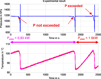
Figure 14. Effect of heating power on the duration of the eruptive cycle, 2.2 m geyser.

Figure 15. An eruptive cycle in a P-T diagram.
During certain phases of the cycle of a geyser (phases 2 - 6 from A to D), there is an equilibrium in the pressure cooker between liquid water and steam. During these phases, the pressure is therefore the saturation vapour pressure, and the (P,T) coordinate points are located on the vaporization curve in the P-T diagram. Between points A and D, the measured points on the P-T diagram should be located on the vaporization curve, which is not the case, except for point C, where the pressure and temperature curves are almost stationary (Figure 12), which gives a vertical tangent (Figure 15). We therefore questioned the temperature sensor’s readings, since the processes take place rapidly between A and D: did it perhaps not have enough time to respond correctly?
ii) Correction of data collected by the temperature sensor.
The temperature sensor only indicates variations in temperature after a certain response time. The experimental data are not therefore accurate, and the sensor output did not correspond to the temperature. It was therefore necessary to take into account the temperature sensor’s response time. To evaluate the sensor’s response time, we conducted a small experiment: we quickly moved the temperature probe from a water bath at room temperature (T = 20.85˚C) to a warmer water bath (T = 40˚C), recording the temperature as a function of time with Latis pro software. We thus obtained the response of the sensor to a temperature step-change. We obtained the recording shown in Figure 16(a). The response curve is reminiscent of a first order system (Figure 16(b)). The black curve shows the real value of the temperature of the water in which the probe is submerged, while the red curve shows the temperature measured by the probe. The green line shows the tangent at the origin, which gives an estimate of the
 (a)
(a) (b)
(b)
Figure 16. Response of the sensor (in red) to a temperature step-change (in black), and associated first order model (b).
time constant τ. The response of the temperature sensor is similar to the response of a first order differential equation system:
(5)
In this equation, τ is the time constant, and a first graphical estimate gives . To obtain a more accurate value, we solve the differential equation when T is a constant:
(6)
To find the most appropriate time constant, we use the least squares method.
We defined the quadratic error, which is a function of the time constant τ:
(7)
k = 0 corresponds to the beginning of the step, and k = kfinal corresponds to the end of the recording.
Using Matlab software, we obtained a plot of the quadratic error (Figure 17). This enabled us to obtain an accurate value for τ which corresponds to the minimum of the quadratic error. Since this minimum is practically zero, we infer that the first order model is a good match.
 (a)
(a) (b)
(b)
Figure 17. Quadratic error as a function of the time constant τ in the model (a); and comparison between output from the model―in black―and output from the sensor―in red―(b).
For the time constant found there is a good match between the model and the experimental result: henceforth, we will conflate the output from the model with the output from the sensor, that is . We can then estimate the temperature from the equation:
(8)
which is feasible if we know . To do this, we carry out the approxima- tion shown in Figure 18(a).
 (a)
(a) (b)
(b)
Figure 18. Approximation of the tangent with the chord (a) and estimate of the temperature (b): raw data (in blue) and data averaged over 9 samples (in pink).
Then:
(9)
And:
(10)
The results are shown in Figure 18(b). The very noisy blue curve is the result of the previous approximation. The noise is due to numerical differentiation, which amplifies the noise in the temperature data. By taking an average over 9 samples, we obtain the pink curve. Filtering thus enables us to obtain a good estimate of the real temperature, and we will now apply this to the experimental data from the pressure cooker.
iii) Second plot of the eruptive cycle with corrected temperature data.
The cycle shown in Figure 19 is obtained with corrected temperature data.
The black curve shows the pressure in the pressure cooker according to the output from the temperature sensor, and the pink curve shows the pressure in the pressure cooker according to the estimated temperature, which is closer to the real temperature. The temperature correction thus enables us to obtain a good match between the model and the experimental data: between the time the steam appears and its complete condensation, both phases are present, and the corresponding points on the P-T diagram are located on the vaporization curve.
We were thus able to understand the cyclical nature of the geyser and show this cycle in the P-T diagram.

Figure 19. An eruptive cycle in the P-T diagram with corrected T data (in pink) and uncorrected T data (in black).
d) Why is there sometimes overpressure at the beginning of an eruption?
In this section we will explain the pressure increase that takes place at the beginning of an eruption when the heating power is high. In Figure 12 this overpressure can be seen between points A and B. To determine its cause we conducted two experiments. (We thought that the presence of water in the column might be preventing the steam produced from escaping sufficiently quickly).
i) Demonstration of overpressure.
On Figure 20(a), two eruptions with the 6 m column are shown: eruption 1, boxed in pink, was carried out normally with a constant heating power of 1.5 kW. Eruption 2, boxed in red, was carried out applying power modulated with
 (a)
(a) (b)
(b)
Figure 20. Eruption 1 with heating and eruption 2 without heating (a); and increase in pressure when the pressure cooker is closed (b).
the On/Off switch, so as to have an eruption that is not heated for the duration of the eruption (once an eruption begins, explosive boiling can no longer be interrupted and it continues even without heating). By observing the formation of bubbles in the transparent tube at the pressure cooker outlet (Figure AIII.1), the onset of eruption can be detected, and the heating can be switched off at the right moment (several trials were necessary). We can see that in eruption 2 there is no overpressure at the start of the eruption, whereas in eruption 1 there is overpressure. The experimental conditions were the same for both eruptions since they were consecutive.
ii) Experiments performed.
We then measured the pressure in the pressure cooker when it was totally closed. We filled the pressure cooker up to the base of the column and plugged the column at its base. We then replaced the safety valve (which is normally triggered at 1.9 bar) and heated the pressure cooker at 1.5 kW. Only the pressure was recordable (Figure 20(b)), and just before reaching 1.9 bar, the pressure measuring hose burst (cf. Annex Figure AIII.4). A point on the curve obtained indicates the hydrostatic pressure for the 6 m geyser.
iii) Digital processing.
We then used digital processing on the data points. We shifted eruption 1 in time to make it begin at exactly the same moment as eruption 2 (at t = 2045 s). The pressure corresponding to eruptions 1 (in pink) and 2 (in red) are shown in Figure 21(a). We then shifted both curves by subtracting 1600 hPa from them (Figure 21(b)). On the same graph we show the pressure of the pressure cooker in Figure 20(b) (pressure cooker closed), also subtracting 1600 hPa from it. The blue curve is the addition of the red curve and the black curve and we obtain the pink curve for the beginning of the eruption. In other words, we have shown that the overpressure at the beginning of the eruption with heating (eruption 1) is the superimposition of the pressure at the start of an eruption without heating (eruption 2) and of the overpressure in the heated closed pressure cooker (without eruption).
e) Depressurization model.
In this section we will model the depressurization of the pressure cooker corresponding to phase 4 in Figure 12. During this phase, liquid water and steam are continuously present in the pressure cooker, which means that the pressure P and temperature T of the water and steam in the pressure cooker are related (vaporization curve equation). We will make the approximation that this curve is a straight line, which means that we can assume that during this phase the variation in enthalpy of the pressure cooker is more or less proportional to the variation in pressure. During phase 4, ignoring heat loss as well as the supply of heat from the hotplate, we can say that the variation in enthalpy of the pressure cooker is solely due to the energy removed via the column. Thus, ignoring the kinetic and potential energy of the steam leaving through the tube, we can therefore write:
 (a)
(a) (b)
(b)
Figure 21. Overpressure at the start of an eruption with heating (in pink) and an eruption without heating (in red), overpressure in the closed pressure cooker (in black). The sum of the red and black curves gives the blue curve.
(11)
where k1 is a proportionality factor that depends on the specific enthalpy of the outgoing steam, the mass of water contained in the pressure cooker during this phase, the specific enthalpy of water, the diameter of the tube and the density of the steam; v is the expulsion speed of the steam.
In addition, the pressure difference ΔP between the pressure cooker and the top of the tube introduces the notion of pressure drops:
(12)
where L is the length of the tube and D its diameter; λ is a coefficient obtained using a Moody chart, which in our situation where everything is fixed (L, D, viscosity of steam) only depends on v; it depends directly on the Reynolds number, which characterizes flow. Thus, at the beginning of phase 4, when the speed is at its highest, λ is greater than towards the end, when we approach the pressure at point C in Figure 12. By combining the two previous equations we obtain with:
(13)
(14)
When integrated, this differential equation simply gives:
for and (15)
It can be seen that the pressure has a parabolic shape locally (since k2, like λ, depends on time). In Figure 22(a) we have shown the first eruption in Figure 8, and we have also plotted in pink the parabola that best describes the fall in P at the end of phase 4 ( and ); in Figure 22(b)―in black―( and ) and―in red―( et ) we have two other shallower parabolas for higher steam expulsion speeds (losses due to friction are therefore smaller, as expected). The dotted pink line shows the pink parabola translated: it shows the slight rise in pressure at the end of phase 5 mentioned in §II.
f) Refilling model.
In this section we will model the replenishment of the pressure cooker after an eruption. This corresponds to phase 6 in Figure 12. Once this phase has begun, we hypothesize that the water from the basin that flows down the column towards the pressure cooker quickly reaches a limiting speed due to friction in the tube. This speed is independent of the height of the model geyser. With τr as the duration of phase 6, replenishment takes place steadily, and, ignoring water mixing dynamics, we can find an approximation to the instantaneous temperature of the pressure cooker on the basis of a heat balance (t is counted from the start of replenishment):
(16)
In this relation, the temperature response depends on the temperature of the
 (a)
(a) (b)
(b)
Figure 22. Parabolic depressurization model: pressure in blue and models in pink, black and red.
basin. In Figure 23(a) we have shown the temperature sensor output in green, the corrected temperature in pink, while the black dashes show the previous model with the experimental conditions of the second eruption in Figure 8(a). Thus M = 8300 g, ΔM = 2500 g, TC = 100 + 273 K, Tbasin = 35 + 273 K, τr = 7.5 s; the model appears to be a good fit, which justifies our hypothesis. In Figure 23(b), we have superimposed all the eruptions in Figure 8 (from the second one onwards), and it can be verified that:
 (a)
(a) (b)
(b)
Figure 23. Replenishment model in phase 6. 2.2 m geyser.
・ replenishment times are more or less the same,
・ the temperature of the basin affects the slope of the temperature.
In Figure 24(a), we have superimposed all the eruptions in Figure 8 (from the second one on), as well as an eruption for a height of 6 m (in blue, with corrected temperature).
Figure 24(b) shows the second eruption in Figure 8, when the temperature in the basin, for the 2.2 m geyser, best corresponds to that of the 6 m geyser. It can be verified that:
 (a)
(a) (b)
(b)
Figure 24. Comparison of a 6 m geyser with a 2.2 m geyser.
・ replenishment time does not depend on the height of the geyser.
・ the previous T(t) model does not depend on the height of the geyser.
・ depressurization at the end of phase 4 for the 6 m geyser corresponds to depressurization for the 2.2 m geyser.
g) Why do some eruptions not lead to the replenishment of the pressure cooker?
In this section we will explain a phenomenon observed during certain eruptions. Looking at Figure 25, we can see the end of a normal eruption followed by
 (a)
(a) (b)
(b)
Figure 25. Effect of heating power on eruption mode (a). End of a normal eruption with replenishment followed by an incomplete eruption (b): continuous boiling without replenishment of the pressure cooker. Pressure (in blue), corrected temperature of the pressure cooker (in pink) and of the basin (in green).
an incomplete eruption: phase 5 in Figure 12 continues without replenishment: there is continuous boiling at a temperature close to 100˚C and a pressure close to 1 bar. The dynamic pressure of the steam leaving the column offsets the hydrostatic pressure of the basin, which prevents another replenishment from taking place. We attempted to quantify this process (see Annex I). To have a normal eruption with filling, it is necessary to have a heating power of:
(17)
We verified experimentally that for a given value of hbasin, a lower heating power (0.83 kW) is not accompanied by an incomplete eruption (Figure 25 experiment with a 1.8 m column), whereas with 1.5 kW we did have one. At t = 3100 s replenishment takes place when the heating power falls from 1.5 kW to 0.83 kW (Figure 25(a)).
3. Conclusions
Thanks to this project, we have improved our understanding of geysers, but that isn’t all. We enjoyed working on this subject because it enabled us to connect our school work to our leisure activities. We love DIY, and this gave us the opportunity to build a model geyser, mainly with recycled materials. We then really enjoyed carrying out the experiments and collecting data so as to find answers to our questions about the phenomena we observed. The main difficulty was that initially we were not able to see anything, either in the column or in the pressure cooker. Thanks to the sensors, which “replaced” our eyes, we were able to collect accurate pressure and temperature data in the model geyser, using a computerized data acquisition system. This allowed us to get an even more detailed understanding of overpressure and certain special regimes, such as the fumarole regime.
We were able to model certain aspects of the geyser cycle, such as its period, depressurization and replenishment. We were lucky enough to be able to talk to researchers about our project and about the various problems we encountered throughout the project. They gave us valuable advice to help us refine our data and our interpretation of it. The project really gave us a desire to continue with our science studies and, indeed, to consider a career as a researcher.
Cite this paper
References
- 1. Bunsen, R. (1847) Physikalische Beobachtungen über die hauptsachlichsten Geisir Islands. [Physical Measurements on an ISLAND Geyser.] Annalen der Physik, 148, 159-170. https://doi.org/10.1002/andp.18471480911
- 2. Lyell, C. (1853) Principles of Geology, or the Modern Changes of the Earth and Its Inhabitants Considered as Illustrative of Geology. J. Murray.
- 3. Tyndall, J. (1870) Heat Considered as a Mode of Motion. D. Appleton.
- 4. Steingisser, A. and Marcus, W. (2009) Human Impacts on Geyser Basins. Yellowstone Science, 17, 7-18.
- 5. Cros, E. (2011) Study of the Dynamics of the Old Faithful Geyser, USA, Using Passive Seismic Methods. Doctoral Thesis, Grenoble.
- 6. Vandemeulebrouck, J., Roux, P. and Cros, E. (2013) The Plumbing of Old Faithful Geyser Revealed by Hydrothermal Tremor. Geophysical Research Letters, 40, 1989-1993. https://doi.org/10.1002/grl.50422
- 7. Steinberg, G.S., Merzhanov, A.G. and Steinberg, A.S. (1981) Geyser Process: Its Theory, Modeling, and Field Experiment. Part 1. Theory of the Geyser Process. Modern Geology, 8, 67-70.
- 8. Steinberg, G.S., Merzhanov, A.G., Steinberg, A.S. and Rasina, A.A. (1981) Geyser Process: Its Theory, Modeling, and Field Experiment. Part 2. A Laboratory Model of a Geyser. Modern Geol, 8, 71-74.
- 9. Teinberg, G.S., Merzhanov, A.G., Steinberg, A.S. and Rasina, A.A. (1981) Geyser Process: Its Theory, Modeling, and Field Experiment. Part 3. On Metastability of Water in Geysers. Modern Geol, 8, 75-78.
- 10. Saptadji, N. and Freeston, D.H. (1991) Laboratory Model of Geysers: Some Preliminary Results. Proceedings 13th Zealand Geothermal Workshop, 155-160.
- 11. Lasič, S. (2006) Geyser Model with Real-Time Data Collection. European Journal of Physics, 27, 995. https://doi.org/10.1088/0143-0807/27/4/031
- 12. Toramaru, A. and Maeda, K. (2013) Mass and Style of Eruptions in Experimental Geysers. Journal of Volcanology and Geothermal Research, 257, 227-239. https://doi.org/10.1016/j.jvolgeores.2013.03.018
- 13. Wang, C.-Y. and Manga, M. (2010) Geysers. In: Earthquakes and Water, Springer Berlin Heidelberg, 117-123.
- 14. Adelstein, E., Tran, A., Saez, C.M., et al. (2014) Geyser Preplay and Eruption in a Laboratory Model with a Bubble Trap. Journal of Volcanology and Geothermal Research, 285, 129-135. https://doi.org/10.1016/j.jvolgeores.2014.08.005
- 15. Brandenbourger, M., Dorbolo, S. and Texier, B.D. (2016) Physics of a Toy Geyser. arXiv preprint arXiv:1603.04925.
- 16. Nechayev, A. (2012) About the Mechanism of Geyser Eruption. arXiv:1204.1560 v1, 13 p.
Annex I:
1) Eruption without replenishment. Complement to paragraph VIII.
During a time interval , the energy supplied to the pressure cooker by the hotplate has the value . This energy is used to vaporize where L is the latent heat of vaporization, which corresponds to a volume:
(18)
and where is the cross-sectional area of the tube and the length of the tube occupied by the volume . This allows us to write:
(19)
At equilibrium, this steam produced will be expelled via the tube in a time interval . It will thus move in which corresponds to a speed:
(20)
This expulsion speed of steam via the tube produces a dynamic pressure which can, if it is sufficient, compensate the hydrostatic pressure
produced by the water of the basin above the top of the tube.
A continuous boiling regime (without replenishment of the pressure cooker) is produced when . We then need a heating power:
(21)
to prevent another replenishment from taking place.
2) Temperature as a sequence. Complement to paragraph III.
In this paragraph we will model the change in the temperature of the cooker along with the successive replenishments of the pressure cooker. In order to do this we use recursive sequences. Thus, each index n corresponds to the end of an eruption. By using the result of §III, we have:
(22)
The temperature of the basin at the end of an eruption depends of course on the temperature of the basin at the end of the previous eruption, of the water received at boiling temperature between T(A) and T(B), and also on the quantity of steam received by the basin during phase 4 (Figure 12) which is of variable duration. Thus we obtain the system:
(23)
We simulated these two sequences with the initial conditions and . The results of these two sequences are marked with stars in Figure AI.1.

Figure AI.1. Comparison of the eruptions of the 2.2 m geyser and of the recursive sequence.
In pink, the temperature of the pressure cooker with the blue stars corresponding to , in green, the temperature of the basin and the red stars corresponding to .
The sequence gives a result which is close to the recorded data. Although the model is quite simple, it needs to be improved for better precision.
Annex II
Details of the experiment with the 6 m column.

Figure AII.1. Counterweight to keep the basin upright.

Figure AII.2. Basin to receive water placed vertically above the pressure cooker.

Figure AII.3. View of the assembly from above.

Figure AII.4. View underneath the basin with the three pipes.

Figure AII.5. Data collection system using Latis pro.

Figure AII.6. Temperature sensor and seals.

Figure AII.7. Overall view of the data collection system.
Annex III
Some images of the eruption of our geyser with a 6 m column.


Figure AIII.1. Steam rises up the column and water gushes out into the basin at the beginning of explosive boiling.

Figure AIII.2. Night-time eruption.

Figure AIII.3. Production of a vortex during depressurization in the pressure cooker.


Figure AIII.4. Measuring pressure in the closed pressure cooker.