Journal of Applied Mathematics and Physics
Vol.07 No.03(2019), Article ID:91448,26 pages
10.4236/jamp.2019.73046
Hematocrit and Slip Velocity Influence on Third Grade Blood Flow and Heat Transfer through a Stenosed Artery
A. Jimoh1, G. T. Okedayo2, T. Aboiyar3
1Department of Mathematical Sciences, Kogi State University, Anyigba, Nigeria
2Department of Mathematical Sciences, Ondo State University of Science and Technology, Okitipupa, Nigeria
3Department of Mathematics/Statistics/Computer Sciences, University of Agriculture, Makurdi, Nigeria

Copyright © 2019 by author(s) and Scientific Research Publishing Inc.
This work is licensed under the Creative Commons Attribution-NonCommercial International License (CC BY-NC 4.0).
http://creativecommons.org/licenses/by-nc/4.0/


Received: November 6, 2018; Accepted: March 25, 2019; Published: March 28, 2019
ABSTRACT
A theoretical investigation concerning hematocrit and slip velocity influence on the flow of blood and heat transfer by taking into account the externally applied magnetic field has been carried out. The mathematical models considered in this work treated blood as a non-Newtonian fluid obeying the third grade fluid model. A suitable geometry of the stenosis is taken into account. Galerkin weighted residual and Newton Raphson methods are used to solve the equations that govern the flow of blood and heat transfer. Analytical expression for the velocity profile, temperature profile, volume flow rate, wall shear stress and resistance to flow were obtained. Graphical representation of results shows that the flow velocity, volumetric flow rate and shear stress increase while resistance to flow and heat transfer rate decrease when the slip velocity increases. Also, flow velocity and volume flow rate decrease while shear stress, heat transfer rate, and resistance to flow increase when the hematocrit parameter increases. Finally, increases in magnetic field parameter lead to decrease in flow velocity, flow rate and shear stress but increase the flow resistance.
Keywords:
Stenosis, Hematocrit, Slip Velocity, Magnetic Field, Non-Newtonian Fluid, Third Grade Fluid, Galerkin Weighted Residual Method

1. Introduction
Atherosclerosis is the deposition or accumulation of cholesterol in the arterial wall and this can cause local narrowing in the lumen of the arterial segment commonly referred to as stenosis. One of the serious consequences, when an obstruction is developed in an artery, is the increased resistance and the associated reduction of the blood flow which can lead to arterial diseases such as stroke, heart attack and serious circulating disorders. Those diseases have been identified as the major causes of death globally (Shanthi et al. [1] ). Since the normal blood flow is disturbed as a result of formation of lumps in the lumen of the arteries, the heat transfers between the living tissues particularly in the peripheral vessels where the temperature is generally closely related with blood flow rate, will also be disturbed. Different studies on blood flow and heat transfer through stenosed arteries have been carried out theoretically and experimentally by several researchers [2] - [10]. Most of these studies considered only the magnetic field effect with no-slip boundary conditions. However, a number of studies of suspensions in general and blood flow in particular have both experimentally (Misra and Shit [11] , Ponalgusamy [12] ), and theoretically (Verma et al. [13] , Guar and Gupta [14] ) suggested the likely presence of slip at the flow boundaries.
In a recent development, Srikanth, et al., [15] investigated blood flow through an overlapping clogged tapered artery in the presence of catheter. They considered velocity slip at the arterial wall since cholesterol deposition is resulting in the stenosis formation. They solved analytically the equation governing the fluid flow under the assumption of mild stenosis. Their results were presented graphically and from the graphs, it was observed that the slip velocity and divergence tapered artery facilitate the fluid flow. The effect of slip velocity on blood flow through an arterial tube in the presence of multiple stenosis was studied by Arun [16]. He considered the effects of length of stenosis and shape parameter on resistance to flow and shear stress. He observed from the graphs that the parameters have small variations for different values of stenosis shape parameter. An approximate perturbation scheme has been adopted by Geeta and Siddique [17] to solve the equations governing the unsteady blood flow through constricted artery in the presence of velocity slip. They characterized the rheology of the blood flow by Bingham plastic fluids model. They considered the important flow parameters such as velocity, flow rate and shear stress and represented the results graphically. They concluded that, since high blood viscosity is very dangerous for the cardiovascular disorders, slip velocity at the stenotic wall may be used as the major tool in reducing the blood viscosity. They also found that the effect of stenosis reduces the flow rate.
All the above mentioned researchers considered only constant viscosity. Variable viscosity of blood dependence on red blood cell concentration (Hematocrit) is another interesting study since the mechanical property of the whole blood depends on the mechanical properties of red blood cell concentration. Hematocrit effect on the axisymmetric blood flow through stenosed arteries has been investigated by Sanjeev and Chandrashekhar [18]. The mathematical model of blood flow through a tapered artery with mild stenosis and hematocrit were studied by Verma and Parihar [19]. Some of the other researchers that considered variable blood viscosity in their studies include Shit and Screenparna [20]; Singh and Rathee [21]; Chitra and Karthikeyan [22]; Jagdish and Rajbala [23].
This paper therefore, is concerned with the problem of investigating hematocrit and slip velocity influence on third grade blood flow and heat transfer through a stenosed artery taking into account the effect of the externally applied magnetic field.
2. Mathematical Models
The equations governing the steady fluid flow and the steady heat transfer as obtained by Mohammed [24] are respectively given as
(2.1)
and
(2.2)
Since we are considering variable viscosity dependent on red blood cell concentration (Hematocrit) we therefore, replace with in (2.1) and (2.2) to respectively obtain
(2.3)
(2.4)
According to Einstein formular for the variable viscosity of blood taken to be
(2.5)
and the hematocrit h(r) is described by Lih [25]
(2.6)
The first term in the LHS of (2.3) can be re-written as
(2.7)
putting (2.5), (2.6) and (2.7) into (2.3) gives
(2.8)
Since we employed velocity slip at the constricted artery as shown in Figure 1 below, the associated slip conditions to (2.8) are

Figure 1. Geometry of the stenosis.
(2.9)
Similarly, the last term in the LHS of (2.4) can be written as:
(2.10)
Substituting (2.5), (2.6) and (2.10) into (2.4) to obtain
(2.11)
The associated slip conditions to (2.11) are:
(2.12)
In order to non-dimensionalize Equations (2.8), (2.9), (2.11) and (2.12), the following parameters and variables were introduced.
(2.13)
Substituting (2.13) into (2.8) and simplified to obtain
(2.14)
where
(2.15)
and the corresponding dimensionless slip conditions to (2.14) can be simplified as
(2.16)
Similarly, substituting (2.13) into (2.11) and simplified to obtain
(2.17)
where,
(2.18)
and the associated slip conditions to (2.17) can be simplified as
(2.19)
and has been described by Young [26] and Biswas [27]
(2.20)
3. Methods of Solution
To obtain the velocity profile to (2.14) using Galerkin weighted residual method, we assume a trial solution of the form
(3.1)
Subjecting (3.1) to the slip conditions (2.16) and simplified to obtain
(3.2)
Let (3.3)
Using (3.3) in (3.2) and simplified to obtain
(3.4)
For convenience sake, we drop the bar and write (3.4) as
(3.5)
From (3.5), we have the followings
(3.6)
(3.7)
(3.8)
(3.9)
(3.10)
(3.11)
The residue for Equation (2.14) can be written as
(3.12)
Taking the shape of the profile (m = 2), using the transformation (3.3) and substituting (3.5), (3.8), (3.10), and (3.11) into (3.12) to obtain
(3.13)
We obtain the weight functions by differentiating (3.5) with respect to and respectively to obtain
(3.14)
and
(3.15)
The following systems were obtained by taking into account the orthogonality of the residue with respect to the weight functions and
(3.16)
(3.17)
When Equations (3.13) and (3.14) are substituted into (3.16), we integrate and simplified to obtain
(3.18)
Similarly, when Equations (3.13) and (3.15) are substituted into (3.17), we integrate and simplified to obtain
(3.19)
By substituting the appropriate values of the parameters ,,,, and N into Equations (3.18) and (3.19), after some rearrangement, we respectively obtained
(3.20)
and
(3.21)
Solving (3.20) and (3.21) using Newton Raphson’s method, we obtained the values of and and when substituted into (3.5) and simplified, we obtained
(3.22)
as the velocity profile of blood flow with hematocrit.
By simulating the appropriate values of the parameters ,,,, and N into (3.18) and (3.19) and follow the same procedures above, we obtain the corresponding values of , and velocity profile w(r). The results are shown in Table 1.
Similarly, to obtained the temperature profile of the heat transfer using Gerlakin’s method, we assume a trial function of the form
(3.23)
Subjecting (3.23) to the slip conditions (2.19) and after simplification we obtain
(3.24)
By using the transformation (3.3) and dropping bar, Equation (3.24) can be written as
(3.25)

Table 1. Values of the parameters used in the numerical results and the corresponding Velocity profile for the blood flow with Hematocrit.
From (3.5) and (3.25) we have
(3.26)
(3.27)
The residue for Equation (2.17) using (3.3) can be written as
(3.28)
Substituting (3.9), (3.26) and (3.27) into (3.28) to obtain
(3.29)
By taking the derivative of (3.25) with respect to and , we obtained the weight functions as obtained in (3.14) and (3.15) respectively.
The following systems are obtained by taking into account the orthogonality of the residue with respect to the weight functions given in (3.14) and (3.15)
(3.30)
(3.31)
Substituting (3.14) and (3.29) into (3.30), we integrate and simplified to obtained
(3.32)
Also, putting (3.15) and (3.29) into (3.31), we integrate and simplified to obtained
(3.33)
Solving the system of non-linear Equations (3.32) and (3.33) using Newton Raphson’s method, we obtained the expression for and as
(3.34)
(3.35)
Substituting the appropriate values of the parameters ,,, and N, and the constants and into (3.34) and (3.35), we obtain the values of and and when substituted into (3.25) and simplified, we obtain
(3.36)
as the temperature profile of the heat transfer with hematocrit.
By simulating the appropriate values of the parameters ,,, and N, and the constants and in (3.34) and (3.35), we obtain the corresponding values of , and which are shown in Table 2.
Volume Flow Rate
The volume flow rate denoted by Q is given by
(3.37)
Putting (3.5) into (3.37) and evaluate to obtain
(3.38)
Shear Stress
The shear stress denoted by is given as
Table 2. Values of the parameters used in the numerical results and the corresponding temperature profile for the heat transfer with hematocrit.
(3.39)
Simplified (3.39) to obtain
(3.40)
Resistance to Flow
The resistance to flow can be denoted as ψ and is given by
(3.41)
4. Results and Discussion
In the previous section we have obtained analytical expressions for different flow characteristics of blood and heat transfer through a stenosed artery under the action of an externally applied magnetic field. In this section we are to discuss the flow and heat transfer characteristics graphically so as to extract useful information difficult or impossible to obtain in the laboratory and also to get a better understanding of physics of the problem under study.
We used Maple 17 computer software to evaluate the analytical results obtained for velocity profiles, temperature profiles, volumetric flow rate, wall shear stress and resistance to flow. In order to observe the quantitative effects of hematocrit parameter, slip velocity, magnetic field parameter, shear shinning, pressure gradient, Eckert number and third grade parameter, we used the results from numerical simulation of the models and these are tabulated in the previous section.
Figures 2-7 shows the variation of velocity profiles along the radial distance for different values of the hematocrit parameter, magnetic field parameter, slip velocity, shear thinning, Reynold number and pressure gradient. It is observed from Figure 1 that the velocity profiles of blood flow decreases significantly as the value of the hematocrit parameter increases. This happen because increase in hematocrit parameter lead to increase in percentage volume of red blood cells and this bring about increase in density and viscosity of the blood flow relatively. Increase in density and viscosity slow down the flow of blood and this causes decreased in velocity of blood significantly. Also, from Figure 2, increases in magnetic field parameter slightly decreases the velocity profile of the blood flow. This is because the Lorentz force which opposes the motion of the blood flow and as a result slow down the flow velocity. It is seen from Figure 4 that velocity profile increases significantly with increase values of the slip velocity. This is because the slip velocity at the stenotic wall reduces the effect of induced magnetic field and viscosity and as such influencing the flow velocity positively. Other parameters that can as well influence the flow significantly are shown in Figures 5-7. We observed from the figures that velocity profile increases with increase values of the shear thinning, Reynold number and pressure gradient.
Figures 8-12 shows the variation of the temperature profiles along the radial distance for different values of the hematocrit parameter, slip velocity, third grade parameter and Eckert number. It is reviewed from Figure 8 that temperature profiles increase with hematocrit parameter because more heat will be generated as the concentration of red blood cells increases. Also, it is seen from Figure 9 that temperature profiles decrease with increases values of the slip velocity. Temperature profiles increase with Eckert number and shear thinning and these are shown in Figure 11 and Figure 12 respectively while decrease with increase in third grade parameter as shown in Figure 10.
Figures 13-15 depicts the effect of hematocrit parameter on volumetric flow rate, shear stress and resistance to blood flow. we observe from the figures that hematocrit parameter increases with shear stress and resistance to flow but reduces the volume flow rate. This happens because high values of hematocrit parameter lead to increases in both low shear rate and blood viscosity and as such reduces the flow rate. Figures 16-18 illustrate the effect of slip velocity on volumetric flow rate, shear stress and resistance to blood flow. It is found that volumetric flow rate and shear stress increase with slip velocity while resistance to flow decreases as slip velocity increases. Variation of volume flow rate, shear stress and resistance to blood flow with magnetic field parameter are illustrated in Figures 19-21. It is seen from Figure 21 that higher values of magnetic field parameter offer more resistance to the flow while volume flow rate and shear stress decreases with increases values of the magnetic field parameter as illustrated in Figure 19 and Figure 20.

Figure 2. Variation of velocity profile of blood along radial distance for different values of hematocrit parameter.

Figure 3. Variation of velocity profile of blood along radial distance for different values of magnetic field parameter.
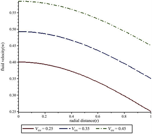
Figure 4. Variation of velocity profile of blood along radial distance for different values of slip velocity.

Figure 5. Variation of velocity profile of blood along radial distance for different values of the shear thinning.

Figure 6. Variation of velocity profile of blood along radial distance or different values of reynold number.

Figure 7. Variation of velocity profile of blood along radial distance for different values of the pressure gradient.

Figure 8. Variation of temperature profile of heat transfer along radial distance for different values of hematocrit parameter.

Figure 9. Variation of temperature profile of heat transfer along radial distance for different values of slip velocity.

Figure 10. Variation of temperature profile of heat transfer along radial distance for different values of third grade parameter.

Figure 11. Variation of temperature profile of heat transfer along radial distance for different values of eckert number.
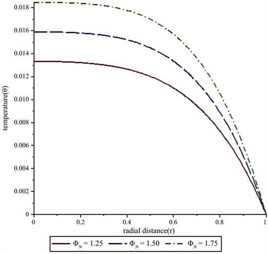
Figure 12. Variation of temperature profile of heat transfer along radial distance for different values of shear thinning.

Figure 13. Variation of volumetric flow rate of blood flow with increasing values of the hematocrit parameter in the entire arterial region along the axial direction.

Figure 14. Variation of shear stress of blood flow with increasing values of the hematocrit parameter in the entire arterial region along the axial direction.

Figure 15. Variation of resistance to blood flow with increasing values of the hematocrit parameter in the entire arterial region along the axial direction.

Figure 16. Variation of volumetric flow rate of blood flow with increasing values of the slip velocity in the entire arterial region along the axial direction.

Figure 17. Variation of shear stress of blood flow with increasing values of the slip velocity in the entire arterial region along the axial direction.

Figure 18. Variation of resistance to blood flow with increasing values of the slip velocity in the entire arterial region along the axial direction.

Figure 19. Variation of volumetric flow rate of blood with increasing values of the magnetic field parameter in the entire arterial region along the axial direction.

Figure 20. Variation of shear stress of blood with increasing values of the magnetic field parameter in the entire arterial region along the axial direction.

Figure 21. Variation of resistance to blood flow with increasing values of the magnetic field parameter in the entire arterial region along the axial direction.
5. Conclusions
In the present analysis, we have studied mathematical models towards investigating the influence of hematocrit and slip velocity on velocity profile, temperature profile, volumetric flow rate, shear stress and resistance to blood flow. Externally applied magnetic field effect was also taken into consideration. Blood is characterized as third grade fluid model. It is observed from the findings that hematocrit parameter significantly reduces the flow velocity and flow rate but increases the wall shear stress, flow resistance and heat transfer rate. The slip velocity significantly increases the flow velocity, flow rate and shear stress but reduces the flow resistance and heat transfer rate. Magnetic field parameter gradually reduces the flow velocity, flow rate and wall shear stress but offers more resistance to blood flow. Also, this study reveals that, elevation of blood hematocrit and blood viscosity are considered as risk factors in the cardiovascular or hemorheological disorder, which can lead to cardiovascular diseases such as heart diseases (myocardial infarction), stroke (cerebrovascular diseases) and hypertension. Similarly, a low range of hematocrit which can lead to more deposition of cholesterol in the endothelium vascular wall is also a risk factor. Since magnetic field opposes the motion of the blood flow, appropriate value of the magnetic field can be used to control blood flow especially in a disease state like hypertension. High rate of heat transfer either as a result of high red blood cells concentrations or environmental factors can cause heat stroke or damage the cells in the body.
Finally, since slip velocity positively influences flow velocity and flow rate, we conclude that device should be suggested for restoring blood flow through the constricted region as well as for reducing the damage to the vessel wall.
Conflicts of Interest
The authors declare no conflicts of interest regarding the publication of this paper.
Cite this paper
Jimoh, A., Okedayo, G.T. and Aboiyar, T. (2019) Hematocrit and Slip Velocity Influence on Third Grade Blood Flow and Heat Transfer through a Stenosed Artery. Journal of Applied Mathematics and Physics, 7, 638-663. https://doi.org/10.4236/jamp.2019.73046
References
- 1. Shanthi, M., Pekka, P. and Norrving, B. (2011) Global Atlas on Cardiovascular Diseases Prevention and Control. World Health Organization in collaboration with world Heart Federation and World Stroke Organisation, 3-18.
- 2. Li, J. and Huang, H. (2010) Effect of Magnetic Field on Blood Flow and Heat Transfer through a Stenosed Artery. Proceedings of 3rd International Conference on Biomedical Engineering and Informatics, Yantai, 16-18 October 2010, 2028-2032. https://doi.org/10.1109/BMEI.2010.5639654
- 3. Alshare, A. Tashtoush, B. and Elkhali, H.H. (2013) Computational Modelling of Non-Newtonina Blood Flow through Stenosed Arteries in the Presence of Magnetic Field. Journal of Biochemical Engineering, 135, 5-15.
- 4. Habibi, M.R. and Ghasemi, M. (2011) Numerical Study of Magnetic Nanoparticles Concentration in Biofluid (Blood) under Influence of High Gradient Magnetic Field. Journal of Magnetism and Magnetic Materials, 321, 32-38.https://doi.org/10.1016/j.jmmm.2010.08.023
- 5. Mekheimer, K.S., Haroun, M.H. and Elkot, M.A (2012) Influence of Heat and Chemical Reactions on Blood Flow through an Isotropically Tapered Elastic Arteries with Overlapping Stenosis. Applied Mathematics, 6, 281-292.
- 6. Sharma, P.R., Sazid, A. and Katiyar, V.K. (2011) Mathematical Modelling of Heat Transfer in Blood Flow through Stenosed Artery. Journal of Applied Sciences Research, 7, 68-78.
- 7. Srinivas, S., Vijayalakshmi, A. and Redely, A.S. (2017) Flow and Heat Transfer of Gold Blood Nanofluid in a Porous Channel with Moving/Stationary Wall. Journal of Mechanics, 33, 395-404.
- 8. Yadav, R.P., Harminder, S. and Bhoopal, S. (2008) Experimental Studies on Blood Flow in Stenosis Arteries in the Presence of Magnetic Field. Ultra Sciences, 20, 499-504.
- 9. Tiari, S., Ahmadpour, M., Tafazzoli-Shadpour, M. and Sadeghi, M.R. (2011) An Experimental Study of Blood Flow in a Model of Coronary Artery with Single and Double Stenosis. Proceedings of the 18th Iranian Conference on Biomedical Engineering, Tehran, 14-16 December 2011, 33-36.
- 10. Aiman, A. and Bourhan, T. (2016) Simulation of MHD in Stenosed Arteries in Diabetic or Anaemic Model. Computational and Mathematical Methods in Medicine, 2016, Article ID: 8123930.
- 11. Misra, J.C. and Shit, G.C. (2007) Role of Slip Velocity in Blood Flow through Stenosed Arteries: A Non-Newtonian Model. Journal of Mechanical in Medicine and Biology, 7, 337-353. https://doi.org/10.1142/S0219519407002303
- 12. Ponalgusamy, R. (2007) Blood Flow through an Artery with Stenosis. A Two Layered Model, Different Shape of Stenosis and Slip Velocity at the Wall. Journal of Applied Sciences, 7, 1071-1077. https://doi.org/10.3923/jas.2007.1071.1077
- 13. Verma, N.K., Siddiqui, S.U., Gupta, R.S. and Mishra, S. (2011) Effect of Slip Velocity on Blood Flow through a Catheterized Artery. Applied Mathematics, 2, 764-770.https://doi.org/10.4236/am.2011.26102
- 14. Guar, M. and Gupta, M.K. (2014) Steady Slip Blood Flow through a Stenosed Porous Artery. Advanced in Applied Sciences Research, 5, 249-259.
- 15. Srikanth, D.S., Ramana, R.S. and Jain, A.K. (2015) Unsteady Polar Fluid Model of Blood Flow through Tapered X-Shape Stenosed Artery. Effect of Catheter and Velocity Slip. Ain Shams Engineering Journal, 6, 1093-1104.https://doi.org/10.1016/j.asej.2015.01.003
- 16. Arun, K.M. (2016) Multiple Stenotic Effect of Blood Flow Characteristic in the Presence of Slip Velocity. American Journal of Applied Mathematics and Statistics, 4, 154-198.
- 17. Geeta, A. and Siddique, S.U. (2016) Analysis of Unsteady Blood Flow through Stenosed Artery with Slip Effect. International Journal of Bio-Science and Bio-Technology, 8, 43-54.
- 18. Sanjeev, K. and Chandraahekhar, D. (2015) Hematocrit Effect of the Axisymmetric Blood Flow through an Artery with Stenosed Arteries. International Journal of Mathematics Trends and Technology, 4, 91-96.
- 19. Verma, N.K. and Parihar, R.S. (2010) Mathematical Model of Blood Flow through a Tapered Artery with Mild Stenosed and Hematocrit. Journal of Applied Mathematics and Computer, 1, 30-46.
- 20. Shit, G.C. and Screeparma, M. (2015) Pulsatile Flow of Blood and Heat Transfer with Variable Viscosity under Magnetic and Vibration Environment. Journal of Magnetism and Magnetic Materials, 388, 106-115.https://doi.org/10.1016/j.jmmm.2015.04.026
- 21. Singh, J. and Rathee, R. (2010) Analytical Solution of Two Dimensional Model of Blood Flow with Variable Viscosity through an Indented Artery Due to LDL Effect in the Presence of Magnetic Field. International Journal of Physical Sciences, 5, 1851-1868.
- 22. Chitra, M. and Karthikeya, D. (2017) Oscillatory Flow of Blood in Porous Vessel of a Stenosed Artery with Variable Viscosity under the Influence of Magnetic Field. International Journal of Innovative Research in Advanced Engineering, 4, 52-60.
- 23. Jagdish, S. and Rajbala, R. (2010) Analytical Solution of Two Dimensional Model of Blood Flow with Varible Viscosity through an Indented Artery due to LDL Effect in the Presence of Magnetic Field. International Journal of Physical Sciences, 5, 1857-1868.
- 24. Mohammed, A.A. (2011) Analytical Solution for MHD Unsteady Flow of a Third Grade Fluid with Constant Viscosity. M.Sc. Thesis, Department of Mathematics, University of Baghdad, Baghdad, 1-104.
- 25. Lih, M.M. (1975) Transport Phenomena in Medicine and Biology. John Willey & Sons, New York, 23.
- 26. Young, D.F. (1968) Effect of Time Dependent Stenosis on Flow through a Tube. Journal of Engineering, 90, 248-254.
- 27. Biswas, D. (2000) Blood Flow Model: A Comparative Study. Mittal Publication, New Delhi, 15.
Nomenclatures
w―Fluid velocity ―Dimensionless fluid velocity
t―Time component ―Dimensionless time component
r―Radial distance y―Dimensionless radial distance
z―Axial distance ―Slip velocity
―Dimensionless Slip velocity for the flow with hematocrit
T―Temperature profile ―Pipe temperature
―Dimensionless temperature profile ―Fluid temperature
―Radius of the normal artery ―Magnetic Field Strength
R(z)―Radius of the artery in a stenotic region ―Electrical Conductivity
―Resistance to flow K―Thermal conductivity
Q―Volumetric flow rate ―Wall Shear Stress
―Maximum height of the stenosis L―Length of the stenosis
N = Hβ = Haematocrit parameter h(r) = Hematocrit at a distance r
= A constant whose value for blood equal 2.5 W = Fluid velocity
(m ≥ 2) = Shape Parameter of Hematocrit
= Viscosity coefficient for plasma
= Coefficient of viscosity of blood at radial distance
―Pressure gradient for the flow with hematocrit
―Slip velocity for the flow with hematocrit
―Magnetic field parameter for the flow with hematocrit
―Shear thinning for the flow with hematocrit
―Eckert number for the heat transfer with hematocrit
―Shear thinning for the heat transfer with hematocrit
―Third grade parameter for the heat transfer with hematocrit