Journal of Applied Mathematics and Physics
Vol.06 No.05(2018), Article ID:84963,25 pages
10.4236/jamp.2018.65094
Acoustic Based Crosshole Full Waveform Slowness Inversion in the Time Domain
Wensheng Zhang1,2, Atish Kumar Joardar1,2,3
1LSEC, ICMSEC, Academy of Mathematics and Systems Science, Chinese Academy of Sciences, Beijing, China
2School of Mathematical Sciences, University of Chinese Academy of Sciences, Chinese Academy of Sciences, Beijing, China
3Department of Mathematics, Islamic University, Kushtia, Bangladesh

Copyright © 2018 by authors and Scientific Research Publishing Inc.
This work is licensed under the Creative Commons Attribution International License (CC BY 4.0).
http://creativecommons.org/licenses/by/4.0/


Received: April 16, 2018; Accepted: May 28, 2018; Published: May 31, 2018
ABSTRACT
We develop a new full waveform inversion (FWI) method for slowness with the crosshole data based on the acoustic wave equation in the time domain. The method combines the total variation (TV) regularization with the constrained optimization together which can inverse the slowness effectively. One advantage of slowness inversion is that there is no further approximation in the gradient derivation. Moreover, a new algorithm named the skip method for solving the constrained optimization problem is proposed. The TV regularization has good ability to inverse slowness at its discontinuities while the constrained optimization can keep the inversion converging in the right direction. Numerical computations both for noise free data and noisy data show the robustness and effectiveness of our method and good inversion results are yielded.
Keywords:
Acoustic Wave Equation, Crosshole, Full Waveform Inversion, Slowness, Bound Constraints, TV Regularization

1. Introduction
Seismic exploration is one of the ways of identifying media properties and structures by propagation of waves. The wave is ignited by sources on the surface and propagates into underground. Due to different properties of media, various waves such as reflection wave and refraction wave are produced. The nature of wave reflection and refraction gives the physical information of media. So the inverse of seismic waves can give geological properties of underground materials. Unlike the observation on the surface, crosshole configuration arranges sources in one well or hole and receivers in another well. Most approaches to the inversion of crosshole data involve traveltime tomography. Traveltime tomography is efficient and robust. However, the resolution of traveltime tomography is limited by its foundation on ray theory and its typical use of first arrivals rather than the full waveform.
The full waveform inversion (FWI) is a high resolution method to inverse the media parameter by using the whole wavefield information such as amplitude, phase and arrival time. The FWI can be divided into two categories, the time- domain method and the frequency-domain method. The FWI was originally developed in the time domain [1] [2] [3] [4] [5] . In 1984, Tarantola [1] laid the foundations for full nonlinear waveform inversion using the formalism of least-squares optimization for the wavefield misfit function. Because of the computational intensity of the forward modelling process, the global optimization methods are impractical. Instead, the gradient-based algorithms are applied to find the local minimum of the misfit function. In 1986, Tarantola [3] extended the theory to elastic wave inversion. The idea was applied to two dimensional crosshole data inversion successfully in the frequency domain [6] [7] [8] [9] . Later much more attentions are paid to the frequency domain method, and the frequency domain method has the same inversion ability like time domain method. Its advantage is that it can be implemented with one selected frequency. However, it needs to solve a large-scale system unlike the time domain method which the forward problem can be implemented effectively in the time domain.
The FWI is a typical ill-posed problem for its nonlinearity and cycle-skipping problem. To overcome the ill-posedness, various methods have been developed, for example the multiscale method [10] [11] [12] and the regularization method [13] [14] . Other methods such as the Laplace-domain method [15] [16] [17] and the envelop FWI method [18] are proposed to improve the inversion robustness. Both the Laplace-domain FWI and envelop FWI are designed to make best of low frequency to enhance the robustness of the inversion. An overview of full waveform inversion can be found in [19] . Driven by potential application, the development of FWI is very rapidly, for example, see [20] [21] [22] .
In this paper, we develop an effective full waveform slowness inversion method for crosshole data by combing the total variation regularization with the constrained optimization together. We also propose the new skip algorithm to implement the constrained optimization problem. The rest of this paper is arranged as follows. The theoretical method is described in Section 2 in detail. It includes the forward method and the inverse method. In Section 3, numerical computations both for the noise free data and noisy date are implemented. Finally, the conclusion is drawn in Section 4.
2. Theory
There are three subsections in this section. In Section 2.1, the forward problem and the staggered-grid scheme with the perfectly matched layer are described. In Section 2.2, the inversion method and the corresponding algorithm by combing TV regularization with bound constraints are described. Section 2.3 involves the computations for the gradient of objective function and the step length, which is important to the success of inversion.
2.1. Forward Method
We consider the acoustic wave equation excited by the source located at the point , which the mathematical form of the pressure satisfies
(1)
(2)
where is the area of computational domain, T is the final observation time, is the square of slowness parameter, v is the wave velocity. The system (1)-(2) is the forward problem. In this paper, we solve the pressure u numerically with the finite difference method for its high computational efficiency. Among various of finite difference schemes, the staggered-grid scheme is a typical one [23] . In order to apply the staggered-grid method, we introduce new variables and defined by and respectively. Then system (1)-(2) can be written as the following hyperbolic form
(3)
(4)
(5)
Now we construct the difference scheme of (3)-(5) on the staggered grids. The schematic map of grid points for different variables is shown in Figure 1. Let be the wavfield at time and position , and be the value at time and position , and so on. Here is the time step, and and are the spatial steps in x and z directions respectively. We approximate Equation (3) at time n and position , Equation (5) at time n and position , and Equation (4) at time and position . Thus we have
(6)
(7)

Figure 1.The schematic map of grid points for the staggered-grid scheme.
(8)
with initial conditions
(9)
(10)
The sufficient and necessary stability for the scheme (6)-(8) is (see Appendix A)
(11)
Since the computational domain is limited, we need to use absorbing boundary conditions to eliminate the boundary reflections. Several methods can be applied, for example, the paraxial approximation [24] , the exact nonreflecting conditions [25] [26] and the perfectly matched layer (PML) method [27] . Here, we adopt the PML method in its split formulation. The idea of PML is to design a particular layer around the computational domain in which the waves will be attenuated satisfactory. In split PML formulation, the wavefield u is split into two components, x-component and z-component, i.e., . To remove the boundary reflections in the absorbing layer, a decaying coefficient or is introduced. Then system (3)-(5) in the case of the source free can be written as the following PML form
(12)
(13)
(14)
(15)
where and are designated to attenuate the refractions in absorbing zone.
We use the following model for the damping parameter [28] [29]
(16)
where L is the thickness of PML absorbing layer, v is the media velocity, x or z is the distance from current position to PML inner boundary, and R is a parameter chosen as . Note that the coefficient is zero in the original computational domain. The staggered-grid scheme for system (12)-(15) is
(17)
(18)
(19)
(20)
(21)
The forward computations can be extrapolated explicitly in the time direction based on (17)-(21). In Figure 2, the snapshot of wave propagation in a homogeneous media with velocity 3000 m/s at time 0.8 s is shown. Figure 2(a) is the result without PML while Figure 2(b) is the result with PML. We can see that the serious boundary reflections in Figure 2(a) are eliminated effectively in Figure 2(b).
2.2. Inversion with Constraints
Consider the inversion of slowness fields in the vector .
 (a)
(a) (b)
(b)
Figure 2.Snapshot of wave propagation at time 0.8 s. (a) No PML; (b) PML.
Define the objective function as
(22)
where the summation is for all the shots or sources in the well. In Equation (22), the first term comes from the misfit between the forward data u and the observed data , the second term is the TV regularization with positive parameter , and is the regularization parameter. The TV regularization is applied because it can yield better inversion result at jump discontinuities theoretically [30] [31] . For more theory about Tikhonov theory, reader may refer to references, for example [32] [33] . The inverse problem is to minimize the objective function, i.e.,
(23)
It is a high dimensional complex optimization problem. The dimensions are , where and are the discretization points along x and z directions respectively. In this paper, the iterative decent method named the global Barzilai-Borwein (GBB) method is applied because it is suitable for solving high-dimensional complex minimization problem [34] [35] [36] . Generally, for a given nonlinear function , let be the initial slowness vector, then the -th iteration is obtained by
(24)
where the superscript m denotes the iteration number, is the step length and is the gradient of at the point .
Now we propose to solve the minimization problem (23) as a constrained optimization problem subject to the constraints . Here a and b are the lower bound and upper bound for each component of the vector σ respectively. The solution of constraint problem for nonlinear optimization is challenging. Usually, the penalty function technique is used to change the constrainted optimization to unconstrained optimization problem [37] . In this paper, we develop a new effective algorithm called the skip method to solve it. The concept of the skip method is to skip the current inverse result if it goes outside of the bound constraints and simply store previous results. For our experience, the skip method performs better than the penalty method. Numerical computations in Section 3 will show the effectiveness of the skip method.
2.3. Computations for the Gradient and Step Length
For minimizing the problem (23), the gradient and the step length are required. The gradient of the objection functional (22) with respect to σ is
(25)
where is the backward wavefield satisfying
(26)
(27)
which can be solved effectively like the forward problem in Section 2.1. The backward problem (26)-(27) is introduced in the gradient derivation naturally in Appendix B. There are two terms on the right hand side of Equation (25). The first is the gradient of the misfit functional between the forward data u and the observed data , which is derived in Appendix B. We remark that there is no Born approximation in the gradient derivation in Appendix B. The second is the gradient of TV regularization term and its discrete form can be obtained by the approximation of the gradient operator, i.e.,
(28)
where
(29)
The parameter in Equation (25) is a small number to prevent the singularity of the denominator.
Now we consider the step length which is important to the success of inversion. For a general objective function :
(30)
the one dimensional line search is applied to find the step length, where is the search direction and is the step length. Line search condition gives the step length which guarantees the sufficient decrease in the objective function by inequality
for some constant . The reduction of the objective function is proportional to both the search direction and the step length. The sufficient condition states that is the step length only if
.
The decrease is not enough if it only satisfies the sufficient condition because it can satisfy for the very small value of . For this reason it requires another essential condition called the curvature condition. If satisfies
for some constant , it is called to satisfy the curvature condition. The sufficient decrease condition and the curvature condition together are called Wolfe condition [37] . It can also be possible a step length satisfies the Wolfe condition but it closes to a minimizer of . Due to this reason we use the modified curvature condition to enlarge the step length which lies in a broad neighbourhood of local minimizer. Therefore, satisfies the strong Wolfe condition if it satisfies the following two conditions
(31)
(32)
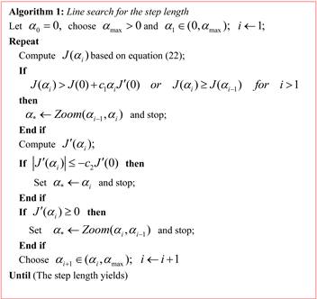
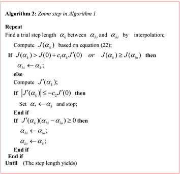
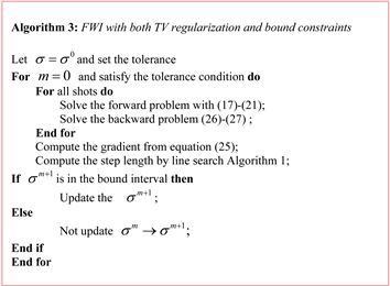
where . For the importance of line search in inversion, the algorithm for line search is given by Algorithm 1 and Algorithm 2. The FWI algorithm with both TV regularization and bound constraints is given by Algorithm 3.
3. Numerical Computations
We implement numerical computations with C-language code. The computational domain is , where and . The spatial increment is and time step . In numerical computations, the regularization parameter is around . The crosshole configuration is shown in Figure 3. The sources are located in the left well marked as * while the receivers are located in the right well marked as o. There are 27 sources in the left well and 29 receivers in the right well. The source function is the Ricker wavelet given by
(33)
where is the peak frequency, A is the maximum amplitude and

Figure 3. The exact slowness model. The sources are in the left well marked as * and the receivers in the right well marked as o.
is the time when maximum amplitude occurs. The squared slowness of the model exact is
(34)
where
.
As shown in Figure 3, this exact model contains a roughly spherical body with lower slowness in the middle on the background media with high slowness. We will consider the inversion in two cases: the noise free data and nosy data.
3.1. Noise Free Data
First we consider the inverse for the noise free data. The inverse result after 54 iterations without TV regularization and bound constraints in Algorithm 3 is shown in Figure 4. We remark that more iterations in Figure 4 is impossible because no step length can be found and the iteration is automatically stopped. We can see the inverse result differs from the exact model very much, which shows the inversion does not converge correctly. The inverse results with three different methods after 200 iterations are shown in Figure 5. For contrast, the exact model is shown in Figure 5(a) again. Figures 5(b)-(d) are the inverse results with TV regularization, with bound constraints, and with both TV regularization and bound constraints, respectively. Comparisons show that Figures 5(b)-(d) are much better than Figure 4. Moreover, Figure 5(d) with both TV regularization and bound constraints is best. Figure 6 is the convergence history

Figure 4. Inverse result without TV regularization and bound constraints. The inversion is stopped automatically after 54 iterations.


Figure 5. Exact model and inverse results with three different methods after 200 iterations. (a) Exact model; (b) TV regularization; (c) Bound constraints; (d) Both TV regularization and bound constraints.
of the objective function for the first 200 iterations. In Figure 6, we can see the curve for the method with both TV regularization and bound constraints

Figure 6. The objective function values for the first 200 iterations.
decreases fastest. The inverse results can be improved further if more iterations are carried out. Figure 7 is a comparison between the exact model and three inverse results after 1000 iterations. Every inversion method takes approximately 12 hours for 1000 iterations with single processor (cpu MHz: 20000.021). Figure 7(a) is the exact model. Figures 7(b)-(d) are the inverse results with TV regularization, with bound constraints, and with both TV regularization and bound constraints, respectively. We can clearly see that Figures 7(b)-(d) are much better than Figures 5(b)-(d), respectively. And Figure 7(d) obtained with both TV regularization and bound constraints performs best. Therefore, the TV regularization and bound constraints are necessary and its effectiveness in inversion is obvious.
3.2. Noisy Data
The recorded data are usually affected by noise due to error in measurements or the influence of natural environment. So it is necessary to consider noise analysis. The Gaussian white noise is one of the effective way to add noise. It has the normal distribution and standard deviation of the data. Let the discrete signal be and the noisy signal . To obtain , we simply add to a white Gaussian noise which is random number with the mean zero and standard deviation under different signal-to-noise ratio (SNR)
(35)
where denotes a normal distribution with mean m and standard derivation , and is the Euclidean mean. We first present some noisy data

Figure 7. Exact model and inverse results with three different methods after 1000 iterations. (a) Exact model; (b) TV regularization; (c) Bound constraints; (d) Both TV regularization and bound constraints.
at different receivers with different SNR levels. Figures 8-10 are the noisy data received from a source with SNR = 100, SNR = 10, SNR = 1, respectively. In each figure, the data received at three different receivers
, i.e.,
,  and
and  are shown. Here
  is the number of discretization points in z direction. In these figures, the red line denotes the noise free data while the blue line represents the noisy data and we can see clearly that the lower SNR is the higher noise in the data. Generally, the inversion for noisy data is challenge because the problem is nonlinear and ill-posed. However, numerical inverse results by our proposed method are still good. In Figure 11, the inverse results by three different methods for noisy data with SNR = 100 are given. Figure 11(a) is the exact model. Figures 11(b)-(d) are the inverse results after 1000 iterations with TV regularization, with bound constraints, and with both TV regularization and bound constraints, respectively. Comparing the results in Figure 11, we can clearly see that Figure 11(d) obtained with both TV regularization and bound constraints performs best. Correspondingly, the inverse results for the noisy data with SNR = 10 and SNR = 1 are shown in Figure 12 and Figure 13 respectively. After comparing these results, we can see that even in the case of lower SNR with SNR = 1, the inverse result with both TV regularization and bound constraints are still good, which shows the robustness of our proposed method.
 (a)
(a) (b)
(b) (c)
(c)
Figure 8. Noisy data with SNR = 100 received in the right well at three different positions . (a)
. (a) , (b)
, (b) , (c)
, (c) .
.
 (a)
(a) (b)
(b) (c)
(c)
Figure 9. Noisy data with SNR = 10 received in the right well at three different positions . (a)
. (a) ; (b)
; (b) ; (c)
; (c) .
.
 (a)
(a) (b)
(b) (c)
(c)
Figure 10. Noisy data with SNR = 1 received in the right well at three different positions . (a)
. (a) ; (b)
; (b) ; (c)
; (c) .
.


Figure 11. Exact model and inverse results with three different methods after 1000 iterations for noisy data with SNR = 100. (a) Exact model; (b) TV regularization; (c) Bound constraints; (d) Both TV regularization and bound constraints.

Figure 12. Exact model and inverse results with three different methods after 1000 iterations f for noisy data with SNR = 10. (a) Exact model; (b) TV regularization; (c) Bound constraints; (d) Both TV regularization and bound constraints.


Figure 13. Exact model and inverse results with three different methods after 1000 iterations for noisy data with SNR = 1. (a) Exact model; (b) TV regularization; (c) Bound constraints; (d) Both TV regularization and bound constraints.
4. Conclusion
Full waveform inversion is an effective method for recovering the media parameter. It is an optimization iterative process by minimizing the misfit between the recorded and synthesized data. In this paper, we have developed a new numerical method for crosshole waveform slowness inversion. This method combines TV regularization with constrained optimization together. The TV regularization method can yield better images of slowness at its discontinuities while the bound constraints from logging data can give more reliable constraints to keep the inversion converging to the right result. The combination is necessary to improve the robustness and inversion precision. The novel skip method is proposed to implement the constrained optimization problem effectively. Numerical computations both for noise free data and noisy data with lower SNR show the effectiveness and robustness of the proposed method. In the future, we will design preconditioners to improve the computational efficiency further.
Acknowledgements
This work is supported by China National Natural Science Foundation under grand number 11471328. It is also supported by the Chinese Academy of Sciences and World Academy of Sciences for CAS-TWAS fellowship and the National Center for Mathematics and Interdisciplinary Sciences, Chinese Academy of Sciences. The computations are completed in the State Key Laboratory of Scientific and Engineering, ICMSEC.
Cite this paper
Zhang, W.S. and Joardar, A.K. (2018) Acoustic Based Crosshole Full Waveform Slowness Inversion in the Time Domain. Journal of Applied Mathematics and Physics, 6, 1086-1110. https://doi.org/10.4236/jamp.2018.65094
References
- 1. Tarantola, A. (1984) Inversion of Seismic Reflection Data in the Acoustic Approximation. Geophysics, 49, 1259-1266. https://doi.org/10.1190/1.1441754
- 2. Gauthier, O., Virieux, J. and Tarantola, A. (1986) Two-Dimensional Nonlinear Inversion of Seismic Waveforms: Numerical Results. Geophysics, 51, 1387-1403. https://doi.org/10.1190/1.1442188
- 3. Tarantola, A. (1986) A Strategy for Nonlinear Inversion of Seismic Reflection Data. Geophysics, 51, 1893-1903. https://doi.org/10.1190/1.1442046
- 4. Mora, P. (1987) Nonlinear Two-Dimensional Elastic Inversion of Multioffset Seismic Data. Geophysics, 52, 1211-1228. https://doi.org/10.1190/1.1442384
- 5. Mora, P. (1988) Elastic Wavefield Inversion of Reflection and Transmission Data. Geophysics, 53, 750-759. https://doi.org/10.1190/1.1442510
- 6. Pratt, R.G. (1990) Frequency-Domain Elastic Wave Modeling by Finite Differences: A Tool for Crosshole Seismic Imaging. Geophysics, 55, 626-632. https://doi.org/10.1190/1.1442874
- 7. Pratt, R.G. and Worthington, M.H. (1990) Inverse Theory Applied to Multi-Source Cross-Hole Tomography, Part 1: Acoustic Wave Equation Method. Geophysical Prospecting, 38, 287-310. https://doi.org/10.1111/j.1365-2478.1990.tb01846.x
- 8. Pratt, R.G. (1990) Inverse Theory Applied to Multi-Source Cross-Hole Tomography, Part 2: Elastic Wave Equation Method. Geophysical Prospecting, 38, 311-329. https://doi.org/10.1111/j.1365-2478.1990.tb01847.x
- 9. Song, Z.M., Williamson, P.R. and Pratt, R.G. (1995) Frequency-Domain Acoustic-Wave Modeling and Inversion of Corsshole Data: Part II Inversion Method, Synthetic Experiments and Real-Data Results. Geophysics, 3, 796-809. https://doi.org/10.1190/1.1443818
- 10. Bunks, C., Saleck, F., Zaleski, S. and Chavent, G. (1995) Multiscale Seismic Waveform Inversion. Geophysics, 60, 1457-1473. https://doi.org/10.1190/1.1443880
- 11. Sirgue, L. and Pratt, R.G. (2004) Efficient Waveform Inversion and Imaging: A Strategy for Selecting Temporal Frequencies. Geophysics, 69, 231-248. https://doi.org/10.1190/1.1649391
- 12. Zhang, W., Luo, J. and Teng, J. (2015) Frequency Multiscale Full-Waveform Velocity Inversion. Chinese Journal of Geophysics, 58, 216-228.
- 13. Signorini, M., Micheletti, S. and Perotto, S. (2016) CMFWI: Coupled Multiscenario Full Waveform Inversion. Inverse Problems in Science and Engineering, 25, 939-964. https://doi.org/10.1080/17415977.2016.1209746
- 14. Guitton, A. (2012) Blocky Regularization Schemes for Full-Waveform Inversion. Geophysical Prospecting, 60, 870-884.
- 15. Shin, C. and Cha, Y.H. (2008) Waveform Inversion in the Laplace Domain. Geophysical Journal International, 173, 922-931. https://doi.org/10.1111/j.1365-246X.2008.03768.x
- 16. Shin, C. and Cha, Y.H. (2009) Waveform Inversion in the Laplace-Fourier Domain. Geophysical Journal International, 177, 1067-1079. https://doi.org/10.1111/j.1365-246X.2009.04102.x
- 17. Ha, T. and Shin, C. (2012) Laplace-Domain Full-Waveform Inversion of Seismic Data Lacking Low-Frequency Information. Geophysics, 77, R199-R206. https://doi.org/10.1190/geo2011-0411.1
- 18. Wu, R.S., Luo, J. and Wu, B. (2014) Seismic Envelop Inversion and Modulation Signal Model. Geophysics, 79, WA13-WA24. https://doi.org/10.1190/geo2013-0294.1
- 19. Virieux, J. and Operto, S. (2009) An Overview of Full-Waveform Inversion in Exploration Geophysics. Geophysics, 74, WCC127-WCC152. https://doi.org/10.1190/1.3238367
- 20. Choi, Y. and Alkhalifah, T. (2018) Time-Domain Full-Waveform Inversion of Exponentially Damped Wavefield Using the Deconvolution-Based Objective Function. Geophysics, 83, R77-R88. https://doi.org/10.1190/geo2017-0057.1
- 21. Manukyan, E., Maurer, H. and Nuber, A. (2018) Improvements to Elastic Full-Waveform Inversion Using Cross-Gradient Constraints. Geophysics, 83, R105-R115. https://doi.org/10.1190/geo2017-0266.1
- 22. Capdeville, Y. and Metivier, L. (2018) Elastic Full Waveform Inversion Based on the Homogenization Method: Theoretical Framework and 2-D Numerical Illustrations. Geophysical Journal International, 213, 1093-1112. https://doi.org/10.1093/gji/ggy039
- 23. Virieux, J. (1986) P-SV Wave Propagation in Heterogeneous Media: Velocity-Stress Finite-Difference Method. Geophysics, 51, 889-901. https://doi.org/10.1190/1.1442147
- 24. Clayton, R. and Engquist, B. (1977) Absorbing Boundary Conditions for Acoustic and Elastic Wave Equations. Bulletin of the Seismological Society of America, 67, 1529-1540.
- 25. Grote, M.J. and Keller, J.B. (2000) Exact Nonreflecting Boundary Condition for Elastic Waves. SIAM Journal on Applied Mathematics, 60, 803-819. https://doi.org/10.1137/S0036139998344222
- 26. Zhang, W., Tong, L. and Chung, E.T. (2014) Exact Nonreflecting Boundary Conditions for Three Dimensional Poroelastic Wave Equations. Communications in Mathematical Sciences, 12, 61-98. https://doi.org/10.4310/CMS.2014.v12.n1.a4
- 27. Berenger, J.P. (1994) A Perfectly Matched Layer for the Absorption of Electromangetic Waves. Journal of Computational Physics, 114, 185-200. https://doi.org/10.1006/jcph.1994.1159
- 28. Collino, F. and Tsogka, C. (2001) Application of the Perfectly Matched Absorbing Layer Model to the Linear Elastodynamic Problem in Anisotropic Heterogeneous Media. Geophysics, 66, 294-307. https://doi.org/10.1190/1.1444908
- 29. Komatitsch, D. and Tromp, J. (2003) A Perfectly Matched Layer Absorbing Boundary Condition for the Second-Order Seismic Wave Equation. Geophysical Journal International, 154, 146-153. https://doi.org/10.1046/j.1365-246X.2003.01950.x
- 30. Royden, R.L. (1968) Real Analysis. 2nd Edition, MacMillan, New York.
- 31. Acar, R. and Vogel, C.R. (1994) Analysis of Total Variation Penalty Methods for Ill-Posed Problems. Inverse Problem, 10, 1217-1229. https://doi.org/10.1088/0266-5611/10/6/003
- 32. Vogel, C.R. (2002) Computational Methods for Inverse Problems. SIAM, Philadelphia.
- 33. Engl, H.W., Hanke, M. and Neubauer, A. (2000) Regularization of Inverse Problems. Kluwer Academic Publishers, Dordrecht/Boston/London.
- 34. Barzilai, J. and Borwein, J. (1988) Two-Point Step Size Gradient Method. IMA Journal of Numerical Analysis, 8, 141-148. https://doi.org/10.1093/imanum/8.1.141
- 35. Raydan, M. (1997) The Barzilai and Borwein Gradient Method for the Large Scale Unconstrained Minimization Problem. SIAM Journal on Optimization, 7, 26-33. https://doi.org/10.1137/S1052623494266365
- 36. Qi, L., Teo, K. and Yang, X. (2005) Optimization and Control with Applications. Springer Science and Business Media, Inc., New York. https://doi.org/10.1007/b104943
- 37. Nocedal, J. and Wright, S. (1999) Numerical Optimization. Springer Science and Business Media, Inc., New York. https://doi.org/10.1007/b98874
Appendix A. The Stability for the Scheme (6)-(8)
We apply the Fourier method to analyze the stability. Since the source term in Equation (8) has no influence on stability, we consider the source-free formulation of the scheme (6)-(8) for brevity, i.e.,
 (36)
(36)
 (37)
(37)
 (38)
(38)
where ,
,  , and
, and  and
and  are the central difference operators in x and z directions respectively. Noting that at time
  we have
 (39)
(39)
Subtracting (39) from (38) and applying (36)-(37), we obtain
 (40)
(40)
Let  and suppose
  and
and  are the wavenumber in the x and z directions respectively. By applying
  to Equation (40), we have
 (41)
(41)
where
 (42)
(42)
 (43)
(43)
and
 (44)
(44)
The sufficient and necessary condition for stability is that the eigenvalues of matrix A is within or on the unit circle. The characteristic equation of matrix A is
 (45)
(45)
The stability requires
 (46)
(46)
which gives
 (47)
(47)
or
 (48)
(48)
which is just the stability (11).
Appendix B. The Derivation for the Gradient
For convenience, we denote the first term in Equation (22) by
 (49)
(49)
and the forward operator A by
 (50)
(50)
where A is given by
 (51)
(51)
The operator A is a self-conjugate operator. See the following Lemma 1.
Lemma 1. For any  satisfying
 (52)
(52)
where  is the Sobolev space, then operator A is the self-adjoint operator, i.e.,
 (53)
(53)
Proof. Based on the definition of the operator A, we have
 (54)
(54)
Applying the Green formula in time and using the conditions (52), the first term in Equation (54) becomes
 (55)
(55)
Similarly, applying the Green formula in space and noting boundary conditions of  and
and , the second term in Equation (54) becomes
 (56)
(56)
Inserting Equations (55) and (56) into Equation (54), we have

The proof is complete. Making variation for the objective function (49), we obtain
 (57)
(57)
where
 (58)
(58)
Note that  and satisfy initial conditions
 (59)
(59)
we obtain  and
and  satisfies
 .
.
Theorem 2 If  is the solution of the following backward problem
 (60)
(60)
 (61)
(61)
then the gradient of the objective function (49) is
 (62)
(62)
Proof Based on Equation (57) and the definition of  by Equations (60)-(61), we have
 (63)
(63)
Using boundary conditions and Lemma 1, we obtain
 (64)
(64)
From the definition we know  and
and  and satisfy
 (65)
(65)
 (66)
(66)
Subtracting Equation (66) from equation (65), we have
 (67)
(67)
Inserting Equation (67) into Equation (64), we have
 (68)
(68)
Let , we obtain the gradient
 (69)
(69)
The proof is completed. The result (69) is just the first term on the right hand side of Equation (25). We can see that there is no Born approximation in the derivation above.