Journal of Applied Mathematics and Physics
Vol.2 No.7(2014), Article ID:46852,13 pages
DOI:10.4236/jamp.2014.27068
The Effect of Time-Stepping on the Accuracy of Green Element Formulation of Unsteady Convective Transport
Okey Oseloka Onyejekwe
Computational Science Program, Addis Ababa University, Arat Kilo Campus, Addis Ababa, Ethiopia
Email: okuzaks@yahoo.com
Copyright © 2014 by author and Scientific Research Publishing Inc.
This work is licensed under the Creative Commons Attribution International License (CC BY).
http://creativecommons.org/licenses/by/4.0/


Received 11 February 2014; revised 11 March 2014; accepted 18 March 2014
ABSTRACT
Despite the significant number of boundary element method (BEM) solutions of time-dependent problems, certain concerns still need to be addressed. Foremost among these is the impact of different time discretization schemes on the accuracy of BEM modeling. Although very accurate for steady-state problems, the boundary element methods more often than not are computationally challenged when applied to transient problems. For the work reported herein, we investigate the level of accuracy achieved with different time-discretization schemes for the Green element method (GEM) solution of the unsteady convective transport equation. The Green element method (a modified BEM formulation) solves the boundary integral theory (A Fredholm integral equation of the second kind) on a generic element of the problem domain in a way that is typical of the finite element method (FEM). In this integration process a new system of discrete equations is produced which is banded and hence amenable to matrix manipulations. This is subsequently deployed to investigate the proper resolution in both space and time for the chosen transient 1D transport problems especially those involving shock wave propagation and different types of boundary conditions. It is found that for three out of the four numerical models developed in this study, the new system of discrete element equations generated for both space and temporal domains exhibits accurate characteristics even for cases involving advection-dominant transport. And for all the cases considered, the overall performance relies heavily on the temporal discretization scheme adopted.
Keywords:Boundary Element Method, Green Element Method, Unsteady Convective Transport Equation, Advection Dominant Transport

1. Introduction
We have chosen to adopt the convection-diffusion equation for this study because of the ubiquitous role it plays in science and engineering fields. Its applications range from groundwater flows, pollutant transport, hydraulics, astrophysics, heat transfer, petrochemistry, chemical engineering, to the transport of momentum and vorticity in fluid flow. Secondly its unique ability to admit either a parabolic or hyperbolic nature offers a very challenging computational experience in numerical analysis.
Little progress has been made towards the analytical solutions of the one-dimensional convection-diffusion equation when initial and boundary conditions become complicated. Hence the existing analytical solutions are limited to problems with simplified boundary or initial conditions [1] [2] . Numerical approaches should therefore be sought for more challenging cases especially where the scalar profiles have been known to exhibit steep gradients in response to Dirichlet outflow boundaries and discontinuities in the boundary conditions; or where severe unphysical oscillations result when grid sizes are not small enough to resolve steep gradients.
The relative simplicity and the basic principles of the ease of formulation of the finite difference method (FDM) is known to attract many followers especially from the engineering community [3] [4] . The common belief that the FDM is capable of solving many problems of engineering interest is reflected on the piles of papers published in this field. However not all these publications emphasize on its reliability and accuracy. It may be surprising that the list of relatively simple, albeit extremely challenging problems that have not been adequately resolved numerically includes the simplest problems of time dependent and convection-dominated problems. Although some of these problems have been used to validate commercial codes, it still remains a mystery how the effects of singularities in the initial and boundary conditions or non-uniformity of the flux profile have been overlooked. Sometimes refinement of time step size or spatial grid size, a common remedy for numerically challenging problems has been known to fail. As a consequence, alternative solution techniques have been sought as a remedy.
A great deal of effort has been devoted to the finite element method (FEM) solution of the convection-diffusion equation. It is well known the standard Gelerkin FEM is not capable of handling some of the difficulties posed by the numerical solution of the convection-diffusion (CD) equation. A combination of standard Galerkin FEM spatial discretization with second-order accurate time approximation schemes such as the Crank-Nicolson, Lax-Wendroff and the leap-frog still fails to perform successfully thus rendering these methods unsuitable for practical applications. A comprehensive account of finite-element-based schemes for CD equation solutions can be found in Morton [5] -[7] and later work by John et al. [8] , Hongfei and Honxing [9] .
Hence well established numerical techniques though reliable for the so called smooth problems can sometimes underperform for the non-smooth ones often encountered in science and engineering. It will be noted that for the particular case of transient problems, the major challenge here does not merely lie in achieving an accurate spatial resolution of the governing CD equation but in guaranteeing an accurate numerical coupling between the spatial and time approximations for a particular problem. Methods for producing reliable numerical results should therefore go beyond the process of introducing extra diffusion effects to damp the unphysical oscillatory behavior of highly convective flows to creating the right balance between spatial and temporal approximations. In this respect, it can be surmised that schemes which employ approximations optimally can enhance the required synergy between spatial and temporal approximations (Taigbenu and Onyejekwe [10] , Onyejekwe [11] ).
A lot has been written about BEM within the past decade due to its rapid spread as a competitive numerical technique, yet more advanced versions of it are needed to deal with field problems of engineering interest. It is well known that for linear potential and steady state problems, BEM ranks as one of the best numerical techniques due to its boundary-only character and ease of formulation. However for transient problems which is our major concern in this paper, domain integration is needed. To prevail over this problem, several versions of BEM have been developed; more importantly, are those based on the theory of particular integrals (Banerjee [12] ) as well as the dual reciprocity boundary element formulations (Wrobel and Brebbia [13] , Power and Patridge [14] and Bulgakov et al. [15] ). Higher order boundary element method involving free space time-dependent fundamental solutions have been used to obtain boundary integral formulation of the transient CD equation (Grigoriev and Dargush [16] ). Despite these attempts, a current review of boundary element literature related to the solution of transient problems still reflects a noticeable decrease in accuracy compared to steady state problems of the same level of complexity and rigor. The reasons for these have not been fully addressed. Moreover it has not been possible except in very few cases [17] [18] to find any work that relates to the existence of certain numerical difficulties that are specific to time dependent BEM formulations. Suffice it to say presently that the boundary-only character of the boundary element theory and its characteristic dimension-reduction capability are not maintained when dealing with transient parabolic/hyperbolic equations or problems subject to singular response arising from non-uniformity of boundary and/or initial conditions. Domain integration oftentimes regarded as an undesirable numerical feature in BEM circles has to be addressed for these types of problems and this often gives rise to surrogate varieties of BEM formulations whose accuracy have not been fully verified for transient transport problems. Competitive efforts along these lines have been recorded by Brebbia and Skerget [19] where they applied the temporal free space Green functions in two spatial dimensions to model the transport equation for low values of Peclet number. Cases for a much wider range of Peclet numbers were handled by Taigbenu and Liggett [20] . The development of an accurate BEM based formulation for time-dependent problems of the CD type and an investigation of the computational difficulties specific to only BEM formulations is a task that is just beginning (Grigoriev [21] , Peratta and Popov [22] ).
To extend the range of applicability of the BEM formulation and especially to deal with the issues related to the numerically difficulties introduced by its encounter with domain discretization for transient problems, we adopt the Green element method (GEM) approach. GEM (Taigbenu [23] ) is rooted in a BEM-FEM formulation and derives a system of discrete element equation based on the singular integral boundary element concept. Its element-by-element formulation promotes its ability to handle not only media heterogeneity (Onyejekwe [24] ) but also transient and nonlinear problems (Onyejekwe [25] ). This approach totally obviates the complexities arising from the use of a two-dimensional boundary element mesh to model a one-dimensional transient problem and hence permits a direct focus on the numerical challenges related to the integral solutions of one-dimensional time-dependent problems.
2. Green Element Formulation
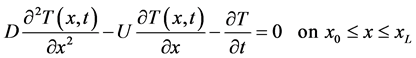
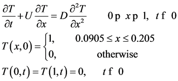
Let us consider the partial differential equation that describes the one-dimensional transport of a scalar in a homogeneous medium under transient fluid flow conditions:
 (1)
(1)
In (1), t is the time, x is the space co-ordinate, T(x,t) is the temperature, U
is the velocity of flow, D is the diffusivity, L is the specific length of the flow
domain Equation (1) governs the transient convective heat diffusion for
 in a one-dimensional domain bounded by two end-points. Both the temperatures T(x,t)
and their fluxes can be specified as Dirichlet and Neumann boundary conditions respectively.
In addition to the boundary conditions, initial conditions can also be specified
at
in a one-dimensional domain bounded by two end-points. Both the temperatures T(x,t)
and their fluxes can be specified as Dirichlet and Neumann boundary conditions respectively.
In addition to the boundary conditions, initial conditions can also be specified
at . For example, the first-type or Dirichlet boundary condition,
specifies the values of the dependent variables at the end-points:
. For example, the first-type or Dirichlet boundary condition,
specifies the values of the dependent variables at the end-points:
 (2a)
(2a)
The second-type or the Neumann-specifies the flux or the spatial derivative of the scalar being transported:
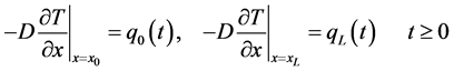 (2b)
(2b)
And the third-type or the so called Cauchy-type boundary condition is a combination of the first and the second-type boundary condition and is given as:
 (2c)
(2c)
where
 are known coefficients. Because of the transient nature of equation (1) an additional
condition must be imposed for the solution to be unique.
are known coefficients. Because of the transient nature of equation (1) an additional
condition must be imposed for the solution to be unique.
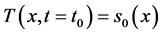 (2d)
(2d)
This condition describes the earlier attained state of equilibrium of the system or the so called initial condition before the beginning of computation. Because of its unique relationship with the problem domain, BEM formulation can no longer be restricted to the problem boundary whenever it is specified.
Our GEM formulation starts by converting the governing differential equation into its integral analog. For the sake of clarity some of the steps given in Taignenu and Onyejekwe [10] will be re-emphasized.
A complimentary differential equation is proposed:
 (3a)
(3a)
where
 is the Dirac delta function and
 is referred to as the source node.
The solution of equation (3a), sometimes referred to as the free-space Green’s function is given by:
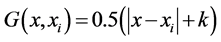 (3b)
(3b)
where k is an arbitrary constant whose value is usually set to the highest length
of an element in the computational domain. We embark on obtaining the integral representation
of equation (1) by invoking one of the Green’s second identities for two functions
 which are at least twice differentiable with respect to the spatial variable namely:
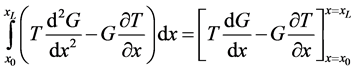 (3c)
(3c)
Equations (1), (3a) and (3b) are substituted into equation (3c) to yield:
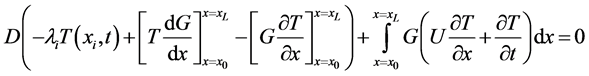 (3d)
(3d)
where the spatial derivative of the free-space Green function is given by :
 (3e)
(3e)
and H the Heaviside function and is defined as:
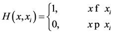


The term
 takes care of the source point Eularian coordinate according to the properties of
the Dirac delta function. For example
takes care of the source point Eularian coordinate according to the properties of
the Dirac delta function. For example
 when the source point
 is within the problem domain
 , and
, and
 when the source point is at
 or
or .
.
It is proper we recognize equation (3d), as a degenerate form of the Fredholm integral
equation and the integral analog of equation (1). Up till now no approximation has
been employed in this elegant BEM integralization procedure. A finite-element-like
solution of equation (3d) is sought for each element of the problem domain. For
a one-dimensional GEM implementation, the solution domain between
 is divided into elements. For M elements, the integral representation of the governing
differential equation can be expressed as the summation of the integral representation
of each of the elements; and equation (3d) can now be written as:
is divided into elements. For M elements, the integral representation of the governing
differential equation can be expressed as the summation of the integral representation
of each of the elements; and equation (3d) can now be written as:
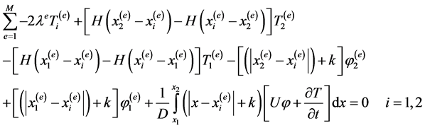 (4a)
(4a)
In order for the line integral over a generic element of the problem domain to be evaluated, we need to interpolate all the functional values within the integral. This is the only step that warrants an approximation in this formulation. For the purposes of this work, we adopt linear interpolating functions to approximate these quantities. For example,
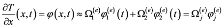
 (4b)
(4b)
where
 stands for the value of the flux
 at the Eularian coordinate
 at time t. A local coordinate system
 with origin at
 is introduced not only to handle the positioning of the source and field nodes within
an element but also to deal with element integration. It is expressed as:
is introduced not only to handle the positioning of the source and field nodes within
an element but also to deal with element integration. It is expressed as: .
.
The element interpolation functions for the case of a 1-D linear element are then
given by: .
.
Interpolation guarantees that the terms within the integral are piecewise continuous
at each node, that is they possess
 continuity. Applying interpolation to the element integral equation yields:
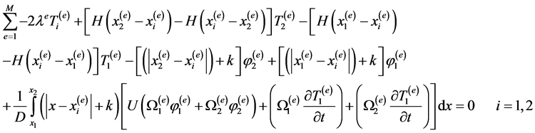 (4c)
(4c)
The flexibility offered by GEM hybrid formulation allows the source node of Equation
(4c) to be related separately to the nodes of a generic element. Placing the source
node
 at the nodes
 or
or
 of an element yields the following equations:
When the source node
 is located at
 Equation (4c) becomes:
 (4d)
(4d)
Similarly for

 (4e)
(4e)
Equations (4d) and (4e) can be written in matrix form as:
 (4f)
(4f)
Without any loss in generality both the summation notation
 and the element counter
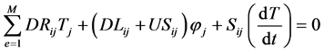
 can now be dropped. Equation (4d) is a system of element first-order linear ordinary
differential equations which can be solved at all the nodes for the primary variable
can now be dropped. Equation (4d) is a system of element first-order linear ordinary
differential equations which can be solved at all the nodes for the primary variable
 and its spatial derivative
 . In order to integrate forward in time
we need to devise an approximation for the time evolution operator.
. In order to integrate forward in time
we need to devise an approximation for the time evolution operator.
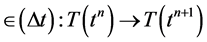 (5a)
(5a)
Equation (5a) allows us to transport the numerical solution at a given time
 to the next time level
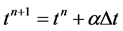 where
where
![]() is a time weighting factor. Equation (4d) can now be written as:
is a time weighting factor. Equation (4d) can now be written as:
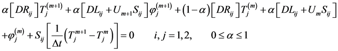 (5b)
(5b)
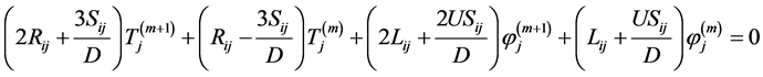
We shall refer equation (5b) as MOD 1. Another approximation of the temporal derivative term which depends on the use of a modified fully implicit time scheme to advance to the next time station is given as:
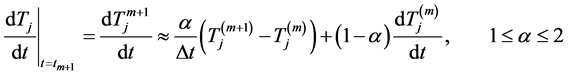 (5c)
(5c)
Adopting the modified fully implicit approximation, equation (4d) can be written as:
 (5d)
(5d)
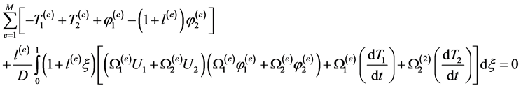
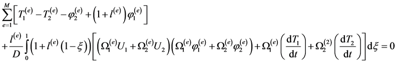
Equation (5d) is referred to as MOD 2. Both MOD 1 and MOD 2 are finite-difference based time approximation schemes. The next approach will explore the integration of equation (4d) in the temporal domain by adopting a FEM-like one-step Galerkin procedure. This aproximation provides another variation of time discretization.
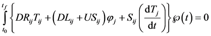 (5e)
(5e)
where
 is a time domain interpolating function. A linear interpolation in the time domain
is adopted for the dependent variable to yield:
is a time domain interpolating function. A linear interpolation in the time domain
is adopted for the dependent variable to yield:
 where:
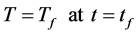
 . After the chores of integration,
the following discrete equation is obtained:
. After the chores of integration,
the following discrete equation is obtained:
 (5f)
(5f)
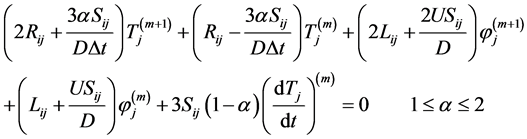
Equation (5f) is known MOD 3. Next, the temporal derivative is approximated implicitly and the discrete equation integrated within the time domain by interpolating the time variable. The resulting discrete equation is given by:
 (5g)
(5g)
where the coefficients are given by:

Equation (5g) is called MOD 4. We may emphasize that although time-dependent discretized equation has been shown before in BEM literature, the numerical implementation of these solutions have often been compromised by inaccuracies resulting from attempts to move back and forth from the problem domain to the boundary and by adopting ad-hoc procedures to deal with the temporal domain. GEM avoids these problems (Taigbenu and Onyejekwe [10] ) by adopting a FEM-like hybrid procedure to handle the problem domain and also by guaranteeing that both the source and the field nodes are situated within the same element.
The numerical formulations developed herein are tested on transport problems of increasing complexity and their overall performance assessed with respect to closed form solutions.
3. Numerical Experiments
Numerical examples of the linear one-dimensional convection-diffusion problems are used to verify the capabilities of the models developed herein. For Problem 1, consider equation (1) with initial and boundary conditions given by:
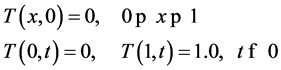 (6a)
(6a)
The analytical solution can be obtained by separation of variables [18] and is given by:
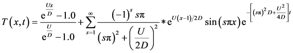 (6b)
(6b)
This problem, is used as a test in [26] and poses a computational challenge at x = 1 where it is characterized by steep boundary layers. In order to highlight the performance of the model formulations, we introduce the finite difference Crank-Nicolson technique. Table 1(a) displays the numerical results and the exact solutions, while Table 1(b) illustrates the error distributions for the four models under study. All the methods are seen to be in agreement with the analytical results for relatively low values of Reynolds numbers.
Four error measurements namely the root-mean-square (rms), the
 and
and
 norms together with the absolute error are used for this study. The
 norm evaluates the maximum nodal-based scalar residual. It is much stricter than
the scalar root-mean-square residuals and indicates the largest error in the computational
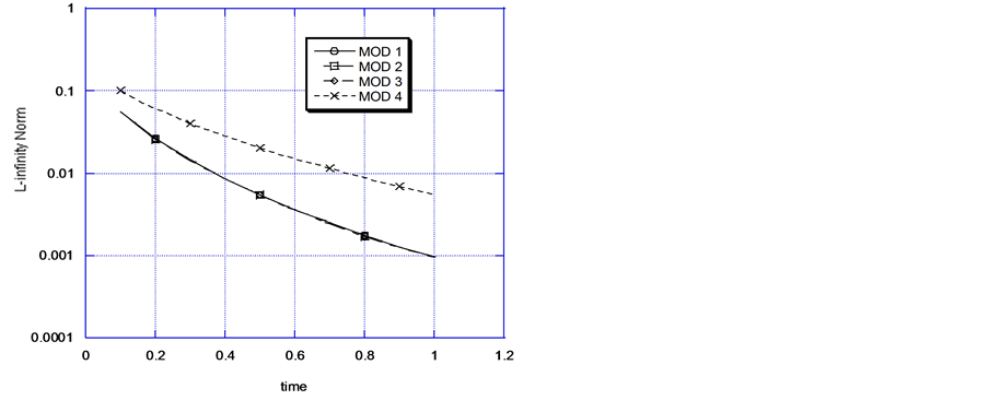
domain for each time step. Figure 1(a) and Figure 1(b) display the temporal error evolution for different
values of Reynolds numbers. Note that Figure 1(a)
shows that MOD 4 performs the best out of the three other models for Re = 1.0. However,
this is not the case for Re = 10.0 where the other three models register lower values
of the
norm evaluates the maximum nodal-based scalar residual. It is much stricter than
the scalar root-mean-square residuals and indicates the largest error in the computational
domain for each time step. Figure 1(a) and Figure 1(b) display the temporal error evolution for different
values of Reynolds numbers. Note that Figure 1(a)
shows that MOD 4 performs the best out of the three other models for Re = 1.0. However,
this is not the case for Re = 10.0 where the other three models register lower values
of the
 norm. Table 1(c) illustrates that a time step size
refinement, a common remedy for smooth problems, does not result in significant
improvement of numerical results as indicated by the magnitudes of the normalized
norm. Table 1(c) illustrates that a time step size
refinement, a common remedy for smooth problems, does not result in significant
improvement of numerical results as indicated by the magnitudes of the normalized
 norm and root-mean-square (rms) error. However it once more confirms the overall
superiority of the other models compared to Model 4 as the value of Re increases.
norm and root-mean-square (rms) error. However it once more confirms the overall
superiority of the other models compared to Model 4 as the value of Re increases.
Problem 1 does not allow a thorough investigation of the ultimate capability that can be attained by any of the models with respect to time and space since little variations in terms of errors are manifested for a greater part of the problem domain. For this reason, we consider another problem with a sharp front gradient (Problem 2):
 (7a)
(7a)
The analytical solution to the above problem is given by:
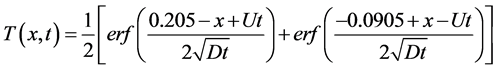 (7b)
(7b)
where the error function is defined as:
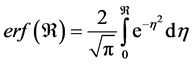 (7c)
(7c)
Table 2 illustrates the performance of all the
models as indicated by various error measurements for different values of Peclet
(Pe) and Courant (Cr) numbers at a stopping time
 It should be noted that no special refinement involving discretization has been
implemented to capture the singular nature of the temperature profile. In addition
care has been taken not to compare results only at selected points located away
from those areas where the scalar profile undergoes discontinuity or to choose a
time where the numerical errors are no longer significant. It is proper to assume
that the largest errors occur in the first time step in the vicinity of the singular
part of the solution profile. We observe that the capability of all the models to
accurately reproduce the solution profile becomes less as the Pe increases. MOD
1, MOD 2 and MOD 3 are significantly more accurate than MOD 4 in terms of the errors
generated. In Figure 2, it can be seen that MOD
4 generates higher errors based on the normalized
It should be noted that no special refinement involving discretization has been
implemented to capture the singular nature of the temperature profile. In addition
care has been taken not to compare results only at selected points located away
from those areas where the scalar profile undergoes discontinuity or to choose a
time where the numerical errors are no longer significant. It is proper to assume
that the largest errors occur in the first time step in the vicinity of the singular
part of the solution profile. We observe that the capability of all the models to
accurately reproduce the solution profile becomes less as the Pe increases. MOD
1, MOD 2 and MOD 3 are significantly more accurate than MOD 4 in terms of the errors
generated. In Figure 2, it can be seen that MOD
4 generates higher errors based on the normalized
 norm
norm . The “kink” observed for all the models shows that integration
is most difficult at small time steps where the solution profile has not yet stabilized.
Note that the rate of increase error is proportional to the increase in time step
for MOD 4. This discrepancy in performance for MOD 4 can be attributed
. The “kink” observed for all the models shows that integration
is most difficult at small time steps where the solution profile has not yet stabilized.
Note that the rate of increase error is proportional to the increase in time step
for MOD 4. This discrepancy in performance for MOD 4 can be attributed
 (a)
(b)
(c)
(a)
(b)
(c)
Table 1 . (a) Numerical solutions Problem 1: Δx = 0.01, Δt = 0.01, Re = 0.01, τ(stoppage time) = 1.0; (b) Comparison of L∞,L2 norms Problem 1: Δx = 0.01, Δt = 0.01, Re = 1.0, τ(stoppage time) = 1.0; (c) Comparison of errors for different parameters of Problem 1: τ(stoppage time) = 1.5.
 (a)
(a)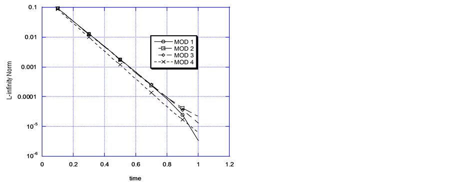 (b)
(b)
Figure 1. (a) Comparison of L∞ errors Δx = 0.01, Δt = 0.01, Re = 1.0, τ(stoppage time) = 1.0; (b) Comparison of L∞ errors Δx = 0.01, Δt = 0.01, Re = 10.0, τ(stoppage time) = 1.0.
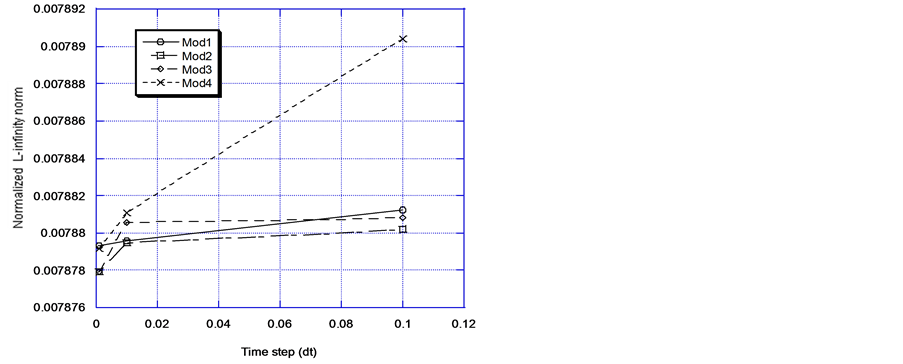
Figure 2. Normalized L∞ norm versus time step.
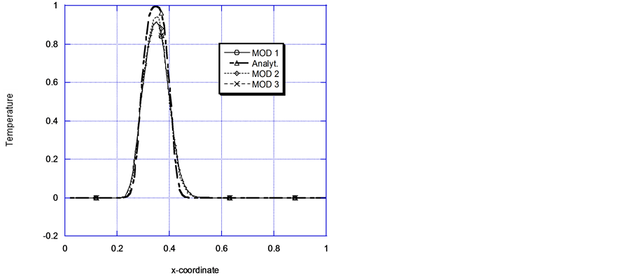
to its approximation of the primary dependent variable in the temporal domain. Figure 3(a) and Figure 3(b) display the performance of the models for different values of Peclet and Courant numbers. For Pe = 10.0 and Cr
Table 2 . Error tests for Problem 2 for different parameters.
 (a)
(a)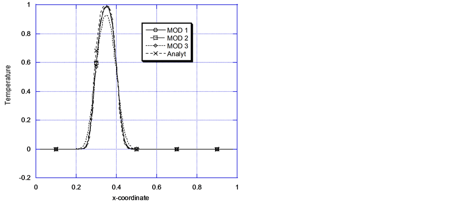 (b)
(b)
Figure 3. (a) Comparison of models solutions Problem 2: Pe = 10, cr = 0.2, τ(stoppage time) = 0.2; (b) Comparison of models solutions Problem 2 Pe = 10, cr = 1.0, τ(stoppage time) = 0.2.
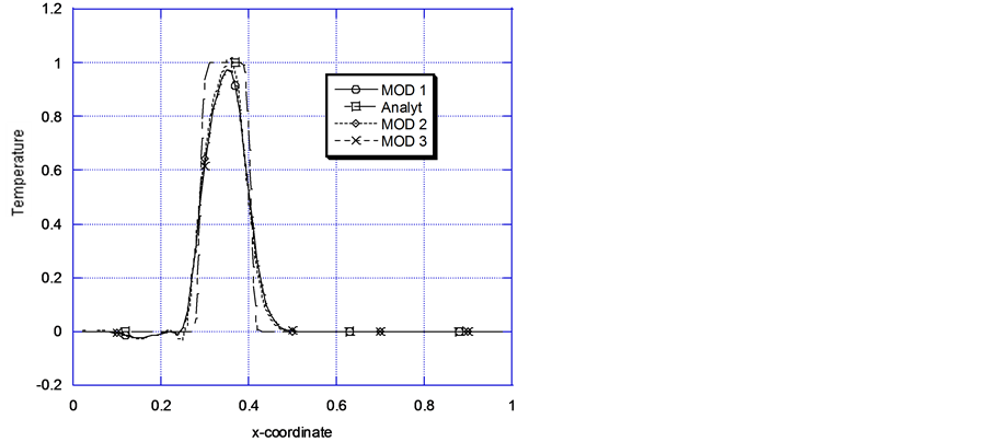
= 0.2 Mod 3 under predicts the solution profile, while MOD 1 and MOD 2 reported very encouraging match of the exact solution. When the Courant number is increased to a value of unity (Cr = 1.0), the propagating characteristics of MOD 1. MOD 2 and MOD 3 become highly modified. They all under predict areas of high gradient with MOD 1 being the most dissipative of the three models. We may mention in passing that for all the results tested so far for Figure 3(a) and Figure 3(b), the numerical solution are free of unphysical spurious oscillations both at the upstream and downstream sections of the concentration solution profile. The three models gave better results for Pe = 10 and Cr = 0.2
Figure 4(a) and Figure
4(b) represent a strongly convection-dominant transport process(Pe = 100).
Even with a Cr = 0.2, Figure 4(a) displays spurious
wiggles, especially for MOD 2 in the region , there is some under prediction in the region
 . Otherwise fairly close results between the numerical and
analytical results are registered for the rest of the problem domain. Figure 4(b) on the other hand shows the influence of the
magnitude of time dicretization on the three models (MOD 1, MOD 2 and MOD 3) for
convection dominant transport. Though MOD 2 still displays oscillatory solutions
in the same region as before and even displays some overshoot, it represents the
best attempt to get as close as possible to the numerical solution.
. Otherwise fairly close results between the numerical and
analytical results are registered for the rest of the problem domain. Figure 4(b) on the other hand shows the influence of the
magnitude of time dicretization on the three models (MOD 1, MOD 2 and MOD 3) for
convection dominant transport. Though MOD 2 still displays oscillatory solutions
in the same region as before and even displays some overshoot, it represents the
best attempt to get as close as possible to the numerical solution.
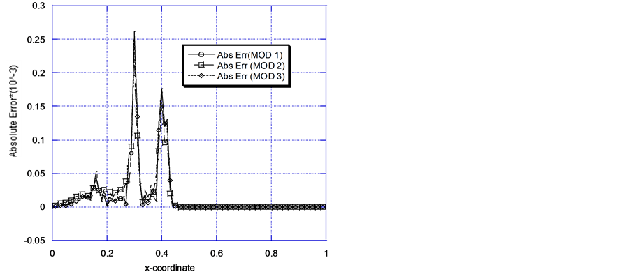
Figure 5(a) and Figure 5(b) display the absolute error evolution for Problem 2. We employ chosen values of Peclet and Courant numbers to visualize the error propagation and characteristics of the three Green element models, MOD 1, MOD 2 and MOD 3. For the test cases we consider two transport modes represented by strongly convection dominant transport processes. We have not focused on the influence of temporal discretization
 (a)
(a)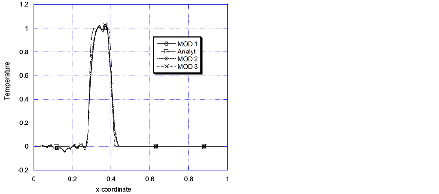 (b)
(b)
Figure 4. (a) Comparison of models solutions problem 2: Pe = 100, cr = 0.2, τ(stoppage time) = 0.2; (b) Comparison of models solutions problem 2: Pe = 100, cr = 1.0, τ(stoppage time) = 0.2.
 (a)
(a)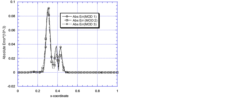 (b)
(b)
Figure 5. (a) Model solutions versus absolute error: Pe = 10, cr = 0.2; (b) Model solutions versus absolute error: Pe = 100, cr = 0.2.
on the numerical solution as represented by the Courant number. This is deliberate. Our major concern here is to see how the models cope with highly convected flows. The Courant number is fixed (Cr = 0.2), the Peclet number is increased from Pe = 10 to Pe = 100. Figure 5(a) represents the case where Pe = 10 and Cr = 0.2. Two distinguishing characteristics are observed namely: there are error-free regions and regions characterized by spikes in absolute error values at the upstream and downstream ends of the problem domain. While the three models are able to accurately represent gradient-free regions of the problem specification, the spikes quantify attempts by the models to handle high gradient areas. While MOD 1 and MOD 3 values of absolute errors are almost identical, MOD 2 can be said to have performed moderately better. When Pe = 100, Cr = 0.2 (Figure 5(b)), the numerical schemes exhibit a trend similar to that of Figure 5(a) except that the spikes are now more pronounced. Convection is more pronounced as the governing equation now tends to be more hyperbolic. It is worthwhile to note the effects of the shockwave propagation and its interaction with the problem boundary conditions. As the shock wave approaches the outflow boundary, the influence of the inflow boundary becomes less significant. On the other hand, when the shockwave encounters the outflow, the zero outflow Dirichlet boundary condition is enforced and the wave recedes upstream. As a result of this interesting physics the numerical error increases dramatically away from the outflow and moves closer to the inflow region. We may mention that the physics becomes significantly different if the problem had admitted infinite boundaries with Neumann boundary conditions or if we had run the problem for long time periods.
4. Conclusion
Boundary element studies related to transient convection diffusion or heat diffusion problems often portray a lack of accuracy that are not usually manifested for the steady state problems. The reasons for this lack of accuracy have neither been properly identified nor been sufficiently investigated in recent boundary element literature except in very few cases [16] [21] . In the work reported herein which points in the direction mentioned above, the commonly used boundary element formulation is hybridized. Based on the singular boundary element theory, the problem domain is discretized in a manner akin to the finite element procedure and a time marching scheme incorporated. Four Green element models (MOD 1, MOD 2, MOD 3, and MOD 4) with different time, approximation schemes have been created to handle convection diffusion transport problems of different degrees of complexity. We note that GEM procedure has been able to deal with some of these computational difficulties in a straightforward manner. While all the models have been able to handle the first problem involving a steep gradient at one of the boundaries for cases involving relatively low values of Reynolds number, MOD 4 was not able to handle a non-smooth problem that is characterized by a sharp front in the problem domain especially for convection dominated transport. Presently significant progress has been made in applying GEM to transient nonlinear flows and this has led to some encouraging results in dealing with transient, nonlinear viscous flows.
Acknowledgements
The author will like to acknowledge the African Institute for mathematical studies (AIMS) Muizenberg South Africa for making their facilities available during the course of this work.
References
- Clearly, R.W. and Ungs, M.J. (1978) Analytical Models for Groundwater Pollution and Hydrology. Report 78-WR-15, Water Resources Program, Princeton University, Princeton.
- van Genuchten, M.Th. and Alves, W.J. (1982) Analytical Solutions of the One-Dimensional Convective-Dispersive Solute Transport Equation. Technical Bulletin 1661, US Department of Agriculture, Washington DC.
- Peaceman, D.W. and Rachford Jr., H.H. (1962) Numerical Calculation of Multi-Dimensional Miscible Displacement. Society of Petroleum Engineers Journal, 2, 327-339
- Price, H.S., Cavendish, J.C. and Varga, R.S. (1968) Numerical Methods of Higher Order Accuracy for ConvectionDiffusion Equations. Society of Petroleum Engineers Journal, 16, 293-300.
- Morton, K.W. (1996) Numerical Solution of Convection-Diffusion Problems. Chapman and Hall, London.
- Li, X.-G. and Chan, C.K. (2004) The Finite Element Method with Weighted Basis Function for Singularly Perturbed Convection Diffusion Problems. Journal of Computational Physics, 195, 773-789. http://dx.doi.org/10.1016/j.jcp.2003.10.028
- Solin, P. (2005) Partial Differential Equations and the Finite Element Methods. John Wiley and Sons. http://dx.doi.org/10.1002/0471764108
- John, V., Mitkhova, T., Roland, M., Sundmacher, K., Tobiska, L. and Voigt, A. (2009) Simulations of Population Balance Systems with One Internal Coordinate Using Finite Element Methods. Chemical Engineering Science, 64, 733-741.
- Fu, H.F. and Rui, H.X. (2012) A Mass-Conservative Characteristic Finite Element Scheme for Optimal Control Governed by Convection-Diffusion Equations. Compt. Methods. Applied Mechanical Engineering, 241, 82.
- Taigbenu, A.E. and Onyejekwe, O.O. (1997) Transient 1D Transport Equation Simulated by a Mixed Green Element Formulation. International Journal for Numerical Methods in Fluids, 25, 437-454.http://dx.doi.org/10.1002/(SICI)1097-0363(19970830)25:4<437::AID-FLD570>3.0.CO;2-J
- Onyejekwe, O.O. (2005) Green Element Method for 2D Helmholtz and Convection-Diffusion Problems with Variable Coefficients. Numerical Methods Partial Differential Equations, 21, 229-241. http://dx.doi.org/10.1002/num.20034
- Banerjee, P.K. (1994) The Boundary Element Methods. McGraw-Hill, London, New York.
- Wrobel, L.C. and Brebbia, C.A. (1987) Dual Reciprocity Boundary Element Formulation for Nonlinear Diffusion Problems. Computer Methods in Applied Mechanics and Engineering, 65, 147-164. http://dx.doi.org/10.1016/0045-7825(87)90010-7
- Power, H. and Patridge, P.W. (1994) “Use of Stokes” Fundamental Solution for the Boundary Only Element Formulation of the Three-Dimensional Navier-Stokes Equations for Moderate Reynolds Numbers. International Journal for Numerical Methods in Engineering, 37, 1825-1840.
- Bulgakov, V., Sarler, B. and Kuhn, G. (1998) Iterative Solution of Systems of Equations in the Dual Reciprocity Boundary Element Method for the Diffusion Equation. International Journal for Numerical Methods in Engineering, 43, 713-732. http://dx.doi.org/10.1002/(SICI)1097-0207(19981030)43:4<713::AID-NME445>3.0.CO;2-8
- Grigoriev, M.M. and Dargush, G.F. (2003) Boundary Element Methods for Transient Convective Diffusion, Part 1: General Formulation and 1D Implementation. Computer Methods in Applied Mechanics and Engineering, 192, 4281-4298.
- Augustin, M., Caiazzo, A., Fiebach, A., Fuhrmann, J., John, V., Linke, A. and Ulma, R. (2011) An Assessment of Discretizations for Convection-Dominated Convection-Diffusion Equations. Computer Methods in Applied Mechanics and Engineering, 200, 3395-3409. http://dx.doi.org/10.1016/j.cma.2011.08.012
- Feng, X.F. and Tian, Z.F. (2006) Alternating Group Explicit Method with Exponential-Type for the Convection-Diffusion Equation. International Journal of Computer Mathematics, 83, 765-775.
- Brebbia, C.A. and Skerget, P. (1984) Diffusion-Convection Problems Using Boundary Elements. In: Liable, J.P., et al., Eds., Proceedings: Finite elements in Water Resources, Springer-Verlag, New York, 747-768. http://dx.doi.org/10.1007/978-3-662-11744-6_63
- Taigbenu, A.E. and Liggett, J.A. (1986) An Integral Solution for the Diffusion-Advection Equation. Water Resources Research, 22, 1237-1246. http://dx.doi.org/10.1029/WR022i008p01237
- Grigoriev, M.M. (2000) Higher-Order Boundary Element Methods for Unsteady Convective Transport. Ph.D. Thesis, Faculty of the Graduate School of the State University of New York, New York.
- Peratta, A. and Popov, V. (2003) Numerical Stability of the BEM for Advection-Diffusion Problems. http://dx.doi.org/10.1002/num.20009
- Taigbenu, A.E. (1995) The Green Element Method. International Journal for Numerical Methods in Engineering, 38, 2241-2263. http://dx.doi.org/10.1002/nme.1620381307
- Onyejekwe, O.O. (1998) A Boundary-Element-Finite-Element Equations Solutions for Flow in Heterogeneous Porous Media. Transport in Porous Media, 31, 293-312. http://dx.doi.org/10.1023/A:1006529122626
- Onyejekwe, O.O. (2012) Combined Effects of Shear and Buoyancy for Mixed Convection in an Enclosure. Advances in Engineering Software, 47, 188-193. http://dx.doi.org/10.1016/j.advengsoft.2011.11.002
- Tian, Z.F. and Yu, P.X. (2011) A High-Order Exponential Scheme for Solving 1D Unsteady Convection-Diffusion Equation. Journal of Computational Mathematics, 235, 2477-2491. http://dx.doi.org/10.1016/j.cam.2010.11.001