Theoretical Economics Letters
Vol. 2 No. 2 (2012) , Article ID: 19296 , 8 pages DOI:10.4236/tel.2012.22034
Hyperbolic Transformation and Average Elasticity in the Framework of the Fixed Effects Logit Model
Faculty of Economics, Kyushu Sangyo University, Fukuoka, Japan
Email: kitazawa@ip.kyusan-u.ac.jp
Received January 13, 2012; revised February 11, 2012; accepted February 20, 2012
Keywords: Fixed Effects Logit; Conditional Logit Estimator; Hyperbolic Transformation; Moment Conditions; GMM; Monte Carlo Experiments; Average Elasticity
ABSTRACT
In this paper, a simple transformation is proposed for the fixed effects logit model, which constructs some valid moment conditions including the first-order condition for one of the conditional MLE proposed by Chamberlain (1980) [1]. Some Monte Carlo experiments are carried out for the GMM estimator based on the transformation. In addition, the average elasticity of the logit probability with respect to the exponential function of explanatory variable is proposed in the framework of the fixed effects logit model, which is computable without the fixed effects.
1. Introduction
Chamberlain (1980) [1] proposes the useful and established estimator for the fixed effects logit model in panel data.1 This estimator is referred to as the conditional logit estimator, which maximizes the likelihood function composed of the probabilities of the (binary) dependent variables conditional on the fixed effects, the (real-valued) explanatory variables, and the intertemporal sums of the dependent variables. The conditional logit estimator is consistent for the situation of small number of time periods and large cross-sectional size, since its conditional likelihood function rules out the fixed effects and accordingly circumvents the incidental parameters problems pointed out by Neyman and Scott (1948) [2].2 This paper advocates another method of consistently estimating the fixed effects logit model for the situation of small number of time periods and large cross-sectional size.3 The procedure of the method is as follows: First, a hyperbolic transformation is applied to the fixed effects logit model with the aim of eliminating the fixed effects. Next, the GMM (generalized method of moments) estimator proposed by Hansen (1982) [20] is constructed by using the moment conditions based on the hyperbolic transformation. It will be seen that these moment conditions include one type of the first-order conditions of the likelihood for the conditional logit estimator. Then, the preferable small sample property of the GMM estimator using the moment conditions based on the hyperbolic transformation is shown by some Monte Carlo experiments.
In addition, this paper presents the calculation formula of the average elasticity of the logit probability with respect to the exponential function of explanatory variable for the fixed effects logit model. The average marginal effect is not obtained due to the incidental parameters problems for the case of the fixed effects logit model with time dimension being strictly fixed, while it seems that no appropriate index measuring the effect of the change of explanatory variable is developed, in author’s best knowledge. Since the average elasticity is able to be calculated using the consistent estimator of the parameter of interest and the average of binary dependent variables without relation to the fixed effects, it can be said that it is a revolutionary index for the fixed effects logit model.
The rest of the paper is as follows: Section 2 presents the implicit form of the fixed effects logit model, the moment conditions based on the hyperbolic transformation, and the GMM estimator. Section 3 illustrates the link between the conditional maximum likelihood estimator (CMLE) mentioned in the first paragraph in this section and the GMM estimator for the case of two periods. Section 4 reports some Monte Carlo results for the GMM estimator. Section 5 presents the average elasticity in the framework of the fixed effects logit model. Section 6 concludes.
2. Fixed Effects Logit Model, Hyperbolic Transformation and GMM Estimator
In this section, the (static) fixed effects logit model is implicitly defined where the error term is of additive form.4 The hyperbolic transformation, which eliminates the fixed effects and then based on which the moment conditions is constructed for estimating the model consistently, is the fruits of the model defined implicitly. The GMM estimator is defined by using the moment conditions constructed. Throughout this paper, the subscripts  and
and  denote the individual and time period respectively, while
  and
and  are number of individuals and number of time periods respectively. Since the short panel is supposed, it is assumed that
  and
and  is fixed. In addition, it is assumed that the variables in the model are independent among individuals.
The fixed effects logit model is able to be written in the implicit form as follows:
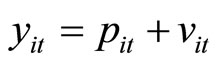 , for
, for ,(2.1)
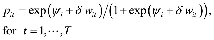 (2.2)
(2.2)
where the observable variables  and
and  are the binary dependent variable and the real-valued explanatory variable respectively, while the unobservable variables
  and
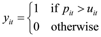
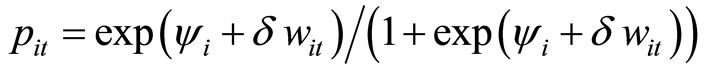
and  are the individual fixed effect and the disturbance respectively.5 Equations (2.1) say that
  take one with probability
 , while it is seen from Equations (2.2) that the probability is the logistic cumulative distribution function of
 . Allowing for the serially uncorrelated disturbances, the uncorrelatedness between the disturbances and the fixed effect and the strictly exogenous explanatory variables, the assumptions on the disturbances are specified as
 , for
, for ,(2.3)
where  for
for ,
,  is defined as the empty set for convenience and
 . The assumptions (2.3) can be derived from the assumption underlying the fixed effects logit model, which is that
  for
for  are mutually independent conditional on
  and
and .6 From now on, based on the fixed effects logit model composed of (2.1) and (2.2) with (2.3), the moment conditions for estimating the parameter of interest
  consistently are constructed by using a hyperbolic transformation, as stated below. Taking notice of the fact that
 (2.4)
(2.4)
and using the formula that
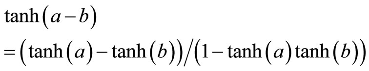 (2.5)
(2.5)
with  and
and  being any real numbers, it follows that
 , (2.6)
where  is the first differencing operator, such as
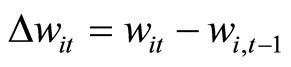 . Since
  and
and  are written as
 (2.7)
(2.7)
and
 (2.8)
(2.8)
respectively by using (2.1) and (2.3), plugging (2.7) and (2.8) into (2.6) gives
 (2.9)
(2.9)
Equations (2.7) and (2.8) are obtained by plugging (2.1) into  and
and
 and then applying (2.3) to them.
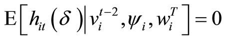
Taking the expectation conditional on  for both sides of (2.9) and then applying law of iterated expectation and (2.3) dated
 , it follows that
 (2.10)
Since  for any positive integer value
  due to the property of binary variable (and accordingly
  and
and ), Equation (2.10) results in
 , for
, for , (2.11)
where
 . (2.12)
The transformation (2.12) is referred to as “the hyperbolic tangent differencing transformation” for the fixed effects logit model in this paper and hereafter abbreviated to “the HTD transformation”.7 It should be noted that as seen from (2.11) and (2.12), observations for which  and
and  make no direct contribution to obtaining the estimates of
  based on the moment conditions (2.11), since
  is invariably zero for these observations.
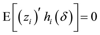
The conditional moment conditions (2.11) give the following  vector of unconditional moment conditions:
 , (2.13)
where 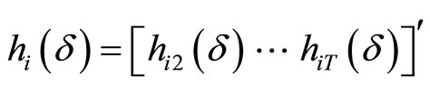 is the
  vector and
 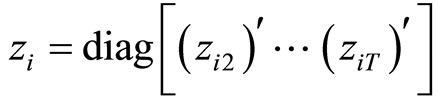 is the
  matrix with
 . The (transposed) blocks
 , for
, for , (2.14)
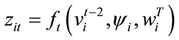
are the  vector-valued functions of
 ,
,  and
and  at time
 , where
  is number of instruments for time
 . By using the empirical counterpart of (2.13):
 (2.15)
and the  inverse of optimal weighting matrix:
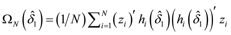 , (2.16)
where  is any initial consistent estimator for
 , the GMM estimator is constructed as follows:
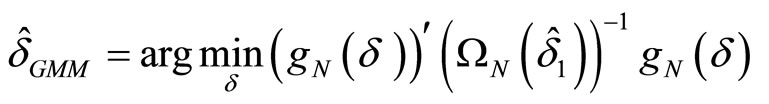 , (2.17)
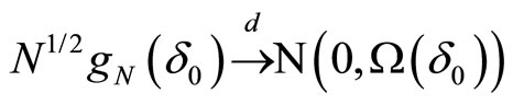
where 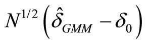 converges in distribution to the normal distribution as follows:
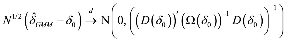 (2.18)
with  being the true value of
 . Taking notice of the assumption that the variables are independent among individuals and adding the assumption that the variables are identically distributed among individuals,
  , which is the (asymptotic) variance-covariance matrix of the moment conditions (2.13), can be written by using
  as follows:
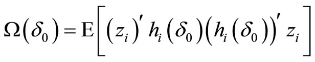 , (2.19)
where it should be noted that (2.16) is the empirical counterpart of (2.19) if  is replaced by
  and
and
 . Further, the first derivative of (2.13) with respect to
  for
for  is as follows:
 . (2.20)
It is conceivable that the discussions for the GMM estimator based on the HTD transformation could be permitted to be conducted on the basis of numbers of observations for which  instead of
 , on the grounds that observations except for those for which
  make no direct contribution to estimating
 .
.
In this case,  is expediently used instead of
  in this section, where
  is number of observations for which
  at time
 .
.
3. Link between CMLE and GMM Estimator
The discussion here is conducted for the case of two periods (i.e.  and
and ). It is shown in this section that the GMM estimator opting for an instrument is identical to the CMLE in this case.
First, the GMM estimator is presented. With  and
and  (both of which are scalars), Equation (2.13) turns to
 . (3.1)
The moment condition (3.1) says that  is used as the instrument for the HTD transformation
 . The GMM estimator for
  is the just-identified one when using only the moment condition (3.1) for the two periods. This is denoted by
  hereafter.
The first derivative of  with respect to
  and the square of
  are respectively calculated as follows:
 (3.2)
(3.2)
and
 (3.3)
(3.3)
where the relationship that  if
if  is even and
  if
if  is odd is used since
  is binary. Using (2.19), (2.20), (3.2), and (3.3),
  and
and  for (3.1) are respectively calculated as follows:
 (3.4)
(3.4)
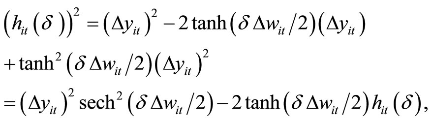
where 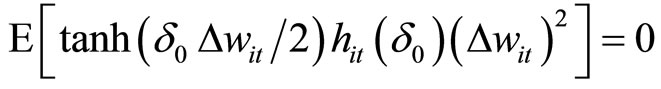 is usedwhich is obtained from (2.11), and
 (3.5)
(3.5)
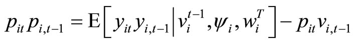
Looking at (3.4) and (3.5), it can be seen that
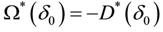 . (3.6)
In addition, the relationship (2.18) is also applicable to the just-identified estimator (see pp. 486-487 in Hayashi, 2000, [23]). Therefore, it follows from (2.18) and (3.6) that the following relationship holds for :
:
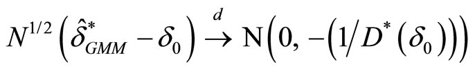 . (3.7)
Lee (2002, pp. 84-87) [24] elucidates the equality conceptually identical to (3.6) in the context of the CMLE to be hereafter described. In addition, Bonhomme (2012) [25] demonstrates that the conditional moment restriction which he proposes for the fixed effects logit model can give birth to the unconditional moment condition identical to (3.1).
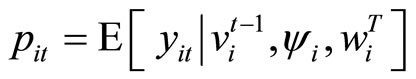
Next, the conventional CMLE proposed by Chamberlain (1980) [1] is presented for the two periods as follows:
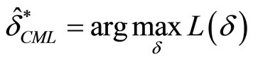 , (3.8)
where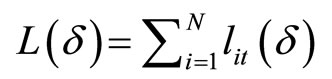 . Referring to Wooldridge
(2002, pp. 490-492) [26], the logarithm of probability composing the conditional log-likelihood function for the two-periods fixed effects logit model is written as follows, with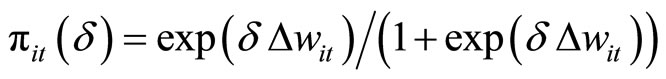 :
:
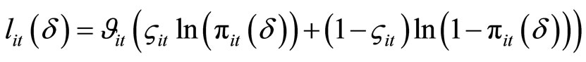 , (3.9)
where  if
if  and
and  otherwise, while
  if
if  and
and  and
and  if
if  and
and . In (3.9),
  stands for the probability with which
  takes one given
 ,
,  ,
,  and
and , while
  stands for the probability with which
  takes zero given
 ,
,  ,
,  and
and .
.
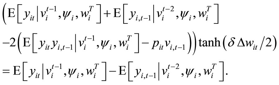
The first-order condition of  is
is
 (3.10)
with
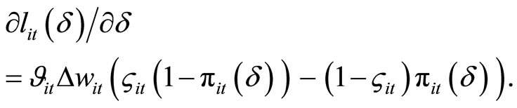 (3.11)
It is corroborated from (3.10) with (3.11) that the first-order condition of  divided by
  is the empirical counterpart of the moment condition (3.1) for the GMM estimator. The second-order derivative of
  with respect to
  is written as
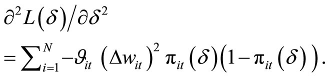 (3.12)
Taking notice of the fact that
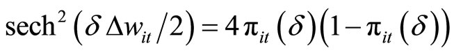 , it is evident that if
  is replaced by
 , (3.12) divided by
  is the empirical counterpart of (3.5) and accordingly identical to
  from (3.6). Therefore, the following relationship holds for
 :
:
 . (3.13)
Judging from the above, it is ascertained that for the two periods the conventional CMLE for the fixed effects logit model is identical to the GMM estimator selecting  as the instrument for the HTD transformation.
To make doubly sure, the integration of
 with respect to
  is conducted:
 (3.14)
where  is the constant of integration. With
  for (3.14), the logarithm of probability (3.9), which composes the conditional log-likelihood function for the two-periods fixed effects logit model, is compactly rewritten as
 (3.15)
The exponential of  in (3.15), which is equivalent to (3.9), represents the probability density when the restriction
 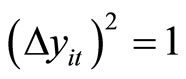 is imposed. In this case, number of observations for which
  is used instead of
  in this section and therefore
 , which is equivalent to
 , could be interpreted as being the asymptotically efficient estimator. This is because the CramérRao inequality is applicable in this case.
Incidentally, Abrevaya (1997) [27] shows that for the fixed effects logit model, a scale-adjusted ordinary maximum likelihood estimator is equivalent to the CMLE for the case of two periods.
4. Monte Carlo
In this section, some Monte Carlo experiments are conducted to investigate the small sample performance of the GMM estimator for the fixed effects logit model described in Section 2. The experiments are implemented by using an econometric software TSP version 4.5 (see Hall and Cummins, 2006, [28]).
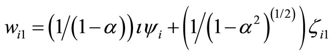
The data generating process (DGP) is as follows:
 ,
,
 ,
,
 ,
,
 ,
,
 ,
,
 ;
; .
.
In the DGP, values are set to the parameters ,
,  ,
,  ,
,  and
and . The experiments are carried out with the cross-sectional sizes
 ,
,  and
and , the numbers of time periods
 ,
,  and
and , and the number of replications
 .
.
In the experiments, the GMM estimator based on the HTD transformation selects  as the instruments for the transformation
 . That is, the GMM(HTD) estimator uses the vector of moment conditions (2.13) with
 , which is able to be written piecewise as follows:
 , for
, for .8 (4.1)
As a control, another GMM estimator is used, which employs the following moment conditions disregarding the unobservable heterogeneity:
 , for
, for . (4.2)
where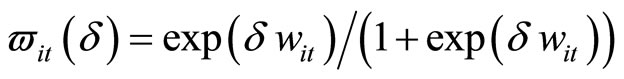 . The GMM (LgtLev) estimator (i.e. the level GMM estimator for the logit model) for
  is inconsistent due to the ignorance of the fixed effects.
The Monte Carlo results are exhibited in Table 1. The settings of values of the parameters for the explanatory variables  are the same as those used by Blundell et al. (2002) [21] for count panel data model. The small sample property of the GMM(HTD) estimator can be said to be preferable and their bias and rmse (root mean squared error) decrease as the cross-sectional size
  increases, which is the reflection of the consistency. In contrast, the sizable downward bias and rmse for the (inconsistent) GMM(LgtLev) estimator remain at virtually constant levels when
  increases. As is seen from comparisons among Simulations (a4), (a8) and (a25), among Simulations (b4), (b8) and (b25), and Simulations (c4), (c8) and (c25) for the GMM(HTD) estimator, the small sample performance of the GMM(HTD) estimator is better off as the number of time periods increases, reflecting the substantive increase of sample size. Furthermore, comparisons among Simulations (a4), (b4) and (c4), among Simulations (a8), (b8) and (c8), and among Simulations (a25), (b25) and (c25) for the GMM(HTD) estimator raise the possibility that more persistent series of the explanatory variables might bring about more deteriorated small sample performance of the GMM(HTD) estimator.9
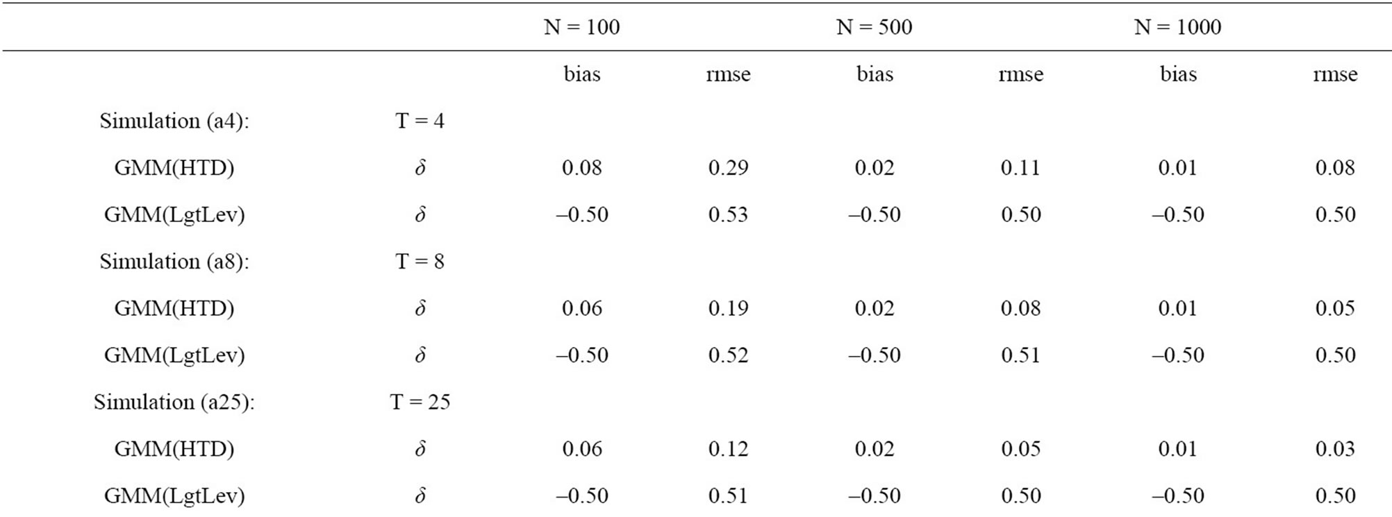
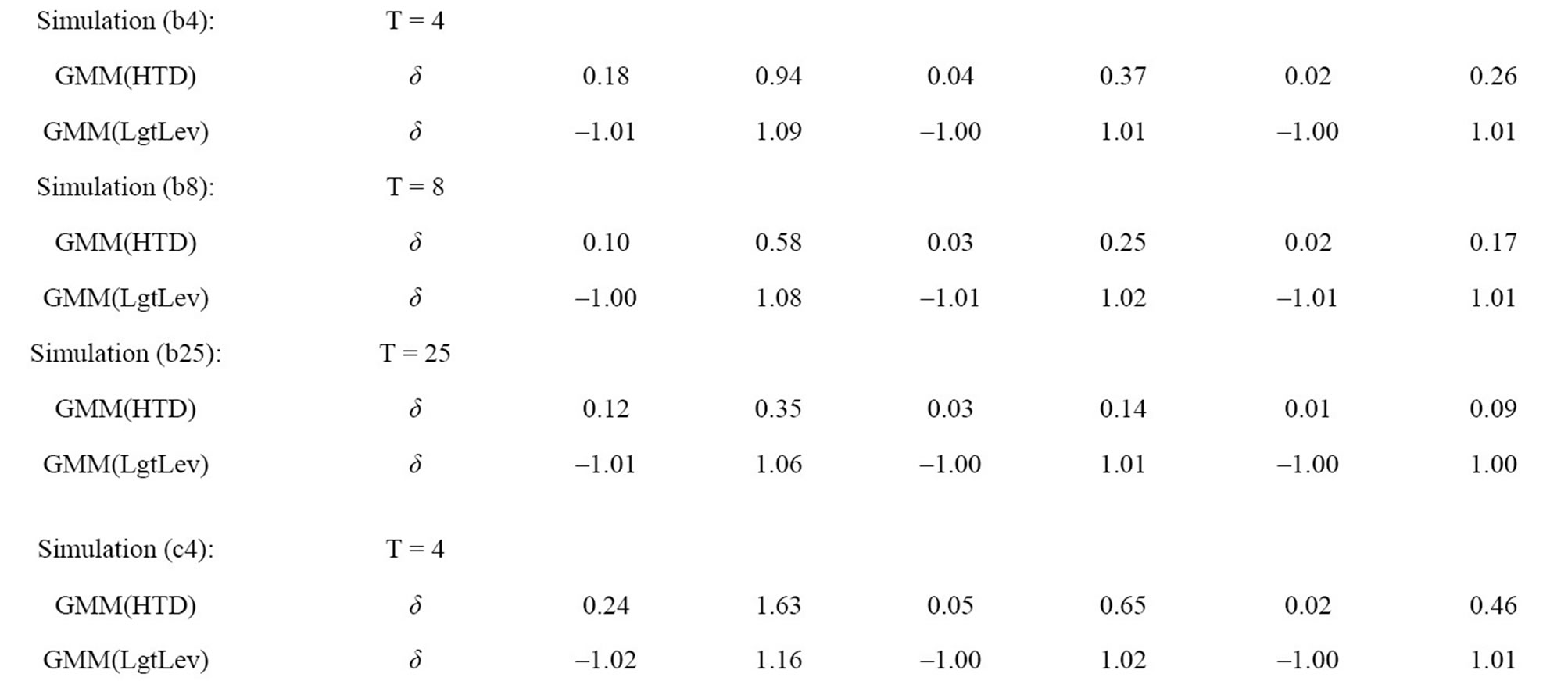
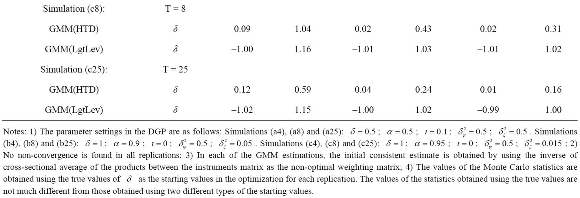
Table 1. Monte Carlo results for the fixed effects logit model.
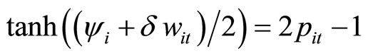
5. Average Elasticity
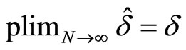
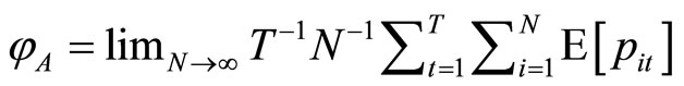
For the fixed effects logit model composed of (2.1) and (2.2), the new index is constructed by using both the consistent estimator for  described in previous sections and the average of
 . The average elasticity of the logit probability with respect to the exponential function of explanatory variable (which is calculated without relation to the fixed effects) is an appropriate index in the framework of the fixed effects logit model with time dimension being strictly fixed, where no (consistent) average marginal effect is available.10 In this section, the assumption that the variables are identically distributed among individuals is unfastened.11
With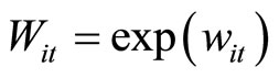 , the elasticity of the probability
  with respect to the positive-valued variable
  (with
(with  being held constant) is defined as follows:
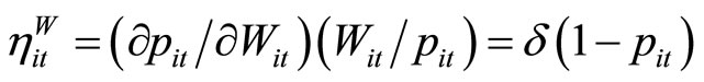 for
for
 . (5.1)
Under the assumption that , the overall average elasticity of
  with respect to
  is calculated with the following formula:
 , (5.2)
where  is the consistent estimator for
  such that
 and
and . Since
 is the probability and
  (and accordingly variances of
  are finite), it can be seen that
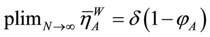 , if
, if
 (which is referred to as the average logit probability in this paper).12
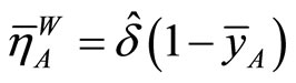
In addition, the cross-section average elasticity for a specific time period and the group average elasticity for a group (e.g. a gender) are able to be calculated as follows, respectively: The formula calculating the cross-section average of  with respect to
  for period
  is
is
 , (5.3)
where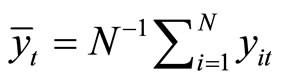 , while that calculating the group average elasticity for group
  in population is
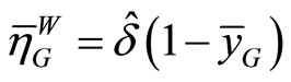 , (5.4)
where 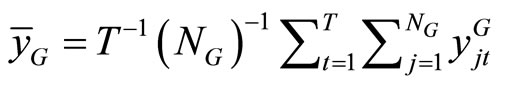 with subscript
denoting the member of group ,
,  being number of individual units belonging to group
 , and
, and  being the binary dependent variable for the individual
  appertaining to group
  at period
 .
.
6. Conclusion
This paper proposed the hyperbolic tangent differencing (HTD) transformation for the fixed effects logit model, with the intention of ruling out the fixed effects. The consistent GMM estimator was constructed by using the HTD transformation. The equivalence of the GMM estimator opting for an instrument and the CMLE proposed by Chamberlain (1980) [1] was revealed for the case of two periods. Then, the Monte Carlo experiments indicated the desirable small sample property of the GMM estimator based on the HTD transformation. In addition, the average elasticity of the logit probability with respect to the exponential function of explanatory variable was proposed, which is an appropriate index from the point of view that it is able to be calculated without the fixed effects. Both of the simple estimator and index will facilitate empirical researchers exploring the binary choice panel data model.
REFERENCES
- G, Chamberlain, “Analysis of Covariance with Qualitative Data,” Review of Economic Studies, Vol. 47, No. 1, 1980, pp. 225-238. doi:10.2307/2297110
- J. Neyman and E. L. Scott, “Consistent Estimates Based on Partially Consistent Observations,” Econometrica, Vol. 16, No. 1, 1948, pp. 1-32.
- G, Rasch, “Probabilistic Models for Some Intelligence and Attainment Tests,” The Danish Institute for Educational Research, 1960.
- G, Rasch, “On General Laws and the Meaning of Measurement in Psychology,” Preceeding of the 4th Berkeley Symposium on Mathematical Statistics and Probability, Vol. 4, 1961, pp. 321-333.
- B. E. Honoré and E. Kyriazidou, “Panel Data Discrete Choice Models with Lagged Dependent Variables,” Econometrica, Vol. 68, No. 4, 2000, pp. 839-874. doi:10.1111/1468-0262.00139
- C. Hsiao, “Analysis of Panel Data,” 2nd Edition, Cambridge University Press, Cambridge, 2003.
- A. Thomas, “Consistent Estimation of Binary-Choice Panel Data Models with Heterogeneous Linear Trends,” Econometrics Journal, Vol. 9, No. 3, 2006, pp. 177-195. doi:10.1111/j.1368-423X.2006.00181.x
- J. Hahn and W. Newey, “Jackknife and Analytical Bias Reduction for Nonlinear Panel Models,” Econometrica, Vol. 72, No. 4, 2004, pp. 1295-1319. doi:10.1111/j.1468-0262.2004.00533.x
- D. R. Cox and N. Reid, “Parameter Orthogonality and Approximate Conditional Inference,” Journal of the Royal Statistical Society, Series B, Vol. 49, No. 1, 1987, pp. 1-39.
- T. Lancaster, “Orthogonal Parameters and Panel Data,” Review of Economic Studies, Vol. 69, No. 3, 2002, pp. 647-666. doi:10.1111/1467-937X.t01-1-00025
- M. Arellano, “Discrete Choices with Panel Data,” Investigaciones Económicas, Vol. 27, No. 3, 2003, pp. 423-458. doi:10.2139/ssrn.261048
- M. Arellano and S. Bonhomme, “Robust Priors in Nonlinear Panel Data Models,” Econometrica, Vol. 77, No. 2, 2009, pp. 489-536. doi:10.3982/ECTA6895
- J, Carro, “Estimating Dynamic Panel Data Discrete Choice Models with Fixed Effects,” Journal of Econometrics, Vol. 140, No. 2, 2007, pp. 503-528. doi:10.2139/ssrn.384021
- I. Fernández-Val, “Fixed Effects Estimation of Structural Parameters and Marginal Effects in Panel Probit Models,” Journal of Econometrics, Vol. 150, No. 1, 2009, pp. 71- 85. doi:10.1016/j.jeconom.2009.02.007
- T. A. Severini, “An Approximation to the Modified Profile Likelihood Function,” Biometrika, Vol. 85, No. 2, 1998, 403-411. doi:10.1093/biomet/85.2.403
- L. Pace and A. Salvan, “Adjustments of the Profile Likelihood from a New Perspective,” Journal of Statistical Planning and Inference, Vol. 136, No. 10, 2006, pp. 3554-3564. doi:10.1016/j.jspi.2004.11.016
- A. Bester and C. Hansen, “A Penalty Function Approach to Bias Reduction in Nonlinear Panel Models with Fixed Effects,” Journal of Business and Economic Statistics, Vol. 27, No. 2, 2009, pp. 131-148. doi:10.1198/jbes.2009.0012
- M. Arellano and J. Hahn, “Understanding Bias in Nonlinear Panel Models: Some Recent Developments,” In: R. Blundell, W. Newey and T. Persson, Eds., Advances in Economics and Econometrics, Cambridge University Press, Cambridge, 2007, pp. 381-409.
- C. Hsiao, “Longitudinal Data Analysis,” In: S. N. Durlauf and E. B. Blume, Eds., Microeconometrics, Palgrave and Macmillan, Basingstoke, 2010, pp. 89-107.
- L. P. Hansen, “Large Sample Properties of Generalized Method of Moments Estimators,” Econometrica, Vol. 50, No. 4, 1982, pp. 1029-1054.
- R, Blundell, R. Griffith and F. Windmeijer, “Individual Effects and Dynamics in Count Data Models,” Journal of Econometrics, Vol. 108, No. 1, 2002, pp. 113-131. doi:10.1016/S0304-4076(01)00108-7
- A. C. Cameron and P. K. Trivedi, “Microeconometrics: Methods and Applications,” Cambridge University Press, Cambridge, 2005.
- F. Hayashi, “Econometrics,” Princeton University Press, Princeton, 2000.
- M. J. Lee, “Panel Data Econometrics,” Academic Press, London, 2002.
- S. Bonhomme, “Functional Differencing,” Econometrica, 2012, in Press.
- J. M. Wooldridge, “Econometric Analysis of Cross-Section and Panel Data,” MIT Press, Cambridge, 2002.
- J. Abrevaya, “The Equivalence of Two Estimators of the Fixed Effects Logit Model,” Economics Letters, Vol. 55, No. 1, 1997, pp. 41-43. doi:10.1016/S0165-1765(97)00044-X
- B. H. Hall and C. Cummins, “TSP 5.0 User’s Guide,” TSP International, 2006.
- R. Blundell and S. Bond, “Initial Conditions and Moment Restrictions in Dynamic Panel Data Models,” Journal of Econometrics, Vol. 87, No. 1, 1998, pp. 115-143. doi:10.1016/S0304-4076(98)00009-8
NOTES
1The rootstock of this estimator is Rasch (1960) [3], (1961) [4].
2Additionally, Honoré and Kyriazidou (2000) [5] propose an estimator for the fixed effects logit model with the lagged dependent variable (as for details, see also pp. 211-216 in Hsiao, 2003 [6]). Further, Thomas (2006) [7] proposes two estimators for the fixed effects logit model with heterogeneous linear trends.
3It seems that the mainstream of late is the development of the biasadjusted estimators, which is available in nonlinear panel data models and aims at the reduction of time-series finite sample bias (i.e. the approximately unbiased estimation of the incidental parameters as well as the parameters of interest, leading to obtaining the approximate marginal effects). Various approaches are proposed in line with the bias-adjustment: Hahn and Newey (2004) [8], Cox and Reid (1987) [9], Lancaster (2002) [10], Arellano (2003) [11], Arellano and Bonhomme (2009) [12], Carro (2007) [13], Fernández-Val (2009) [14], Severini (1998) [15], Pace and Salvan (2006) [16], Bester and Hansen (2009) [17], etc. Some of the approaches are reviewed in Arellano and Hahn (2007) [18] and Hsiao (2010) [19]. However, author’s policy is to conduct the consistent estimation for the case of small time dimension and therefore this paper is not bent upon the bias-adjusted estimators.
4The regression form defined implicitly is also used by Blundell et al. (2002) [21] for count panel data.
5It is generally assumed that the individual effect  is correlated with the explanatory variables
  for each
 .
.
6If the underlying assumption holds, the following relationship is obtained: , where
  is the conditional probability density function and
 . Accordingly, it follows that
 . As for details, see p. 23 in Cameron and Trivedi (2005) [22]. Taking notice of (2.1) and the fact that
 , the assumptions (2.3) are obtained.
7If the much weaker assumptions  for
for  are used instead of (2.3), the moment conditions
  for
for  can be obtained instead of (2.11), where
  and
and  is defined as the empty set for convenience. It should be noted that under the assumptions
  for
for , the (consistent) CMLE proposed by Chamberlain (1980) [1] is no longer obtained for
 . The implication of
  is that although the decision
  wields no influence over the explanatory variable
  just behind its decision, it can make some sort of influences on the explanatory variables after
 , while that of (2.3) is that the decision
  have no influence on the explanatory variables after its decision. In addition, it is regrettable that at this stage, author is unable to construct the valid moment conditions when
  is endogenous. This would be a task for the future.
8Since the moment conditions (4.1) are valid even under the assumptions  for
for , the usage of the GMM (HTD) estimator using the moment conditions (4.1) is generally more conservative than that of the CMLE proposed by Chamberlain (1980) [1] (see footnote 7 in section 2). The CMLE is inconsistent under the assumptions
  for
for  and
and .
.
9This possibility is also pointed out in the framework of ordinary and count panel data models. For example, see Blundell and Bond (1998) [29] and Blundell et al. (2002) [21].
10Frequently, the explanatory variables in the fixed effects logit model are logarithmically transformed.
11In this case, (2.19) and (2.20) in Section 2 are replaced by  and
and , respectively. The same is applied to (3.4) and (3.5) in Section 3.
12Just in case, it is assumed that both  and
and  exist for each
  and
and . However, author thinks that it seems that this assumption is satisfied in any case.