Journal of Mathematical Finance
Vol.06 No.01(2016), Article ID:63856,22 pages
10.4236/jmf.2016.61014
The Effects of Long Memory in Price Volatility of Inventories Pledged on Portfolio Optimization of Supply Chain Finance
Juan He1,2, Jian Wang1,2, Xianglin Jiang3
1School of Transportation & Logistics, Southwest Jiaotong University, Chengdu, China
2Laboratory for Supply Chain Finance Service Innovation, Southwest Jiaotong University, Chengdu, China
3Institute for Financial Studies, Fudan University, Shanghai, China

Copyright © 2016 by authors and Scientific Research Publishing Inc.
This work is licensed under the Creative Commons Attribution International License (CC BY).
http://creativecommons.org/licenses/by/4.0/


Received 2 December 2015; accepted 23 February 2016; published 26 February 2016
ABSTRACT
Due to the illiquidity of inventories pledged, the essential of price risk management of supply chain finance is to long-term price risk measure. Long memory in volatility, which attests a slower than exponential decay in the autocorrelation function of standard proxies of volatility, yields an additional improvement in specification of multi-period volatility models and further impact on the term structure of risk. Thus, long memory is indispensable to model and measure long-term risk. This paper sheds new light on the impact of the existence and persistence of long memory in volatility on inventory portfolio optimization. Firstly, we investigate the existence of long memory in volatility of the inventory returns, and examine the impact of long memory on the modeling and forecasting of multi-period volatility, the dependence structure between inventory returns and portfolio optimization. Secondly, we further explore the impact of the persistence of long memory in volatility on the efficient frontier of inventory portfolio via a data generation process with different long memory parameter in the FIGARCH model. The extensive Monte Carlo evidence reveals that both GARCH and IGARCH models without accounting for long memory will misestimate the actual long-term risk of the inventory portfolio and further bias the efficient frontier; besides, through A sensitive analysis of long memory parameter d, it is proved that the portfolio with higher long memory parameter possesses higher expected return and lower risk level. In conclusion, banks and other participants will benefit from the long memory taken into the long-term price risk measure and portfolio optimization in supply chain finance.
Keywords:
Supply Chain Finance, Long Memory, Long-Term Risk Measure, Portfolio Optimization

1. Introduction
As a significant part at the intersection of supply chain management and trade finance, supply chain finance (SCF) has become one of the hottest topics in business administration [1] . SCF is the inter-company optimization of financing as well as the integration of financing processes with customers, suppliers, and service providers in order to increase the value of all participating companies [2] . It aims to close the gap between our knowledge on product and information flow oriented innovations and financial flow innovations along the supply chain [3] . The spectrum of SCF ranges from pre-shipment financing like raw material financing, purchase-order financing, in- transit inventory financing like vendor-managed inventory finance, third party inventory finance to post-shipment financing like receivables financing, early payment discount programs and payables extension financing [4] .
In China, SCF somewhat differs from western countries like America, Europe, which is a sort of pledge business performed by banks, focal companies, SMEs (small & medium enterprises), logistics companies and so on. Besides, the pledges are mainly the inventories traded in the spot commodity market (such as raw materials, half-finished products and products) rather than the widely-used rights pledges (receivables financing, payables financing and derivatives) in developed countries. In conclusion, SCF in China takes form of inventory financing or logistics financing. It is not only an extended business of modern logistics, but more importantly, helps to solve the financing predicament problems of many SMEs. According to CSCMP China (Council of Supply Chain Management Professionals China), the amount of financing balance of SCF will reach 15,000 billion Yuan RMB in 2020. Although the potential of SCF in China is immense; it faces various complex challenges, especially the credit risk management of borrowers.
In SCF practice of China, pledged inventories play a crucial role in mitigating credit risk of SMEs. In the cases of credit risk of SMEs, lenders’ loss can be reduced by selling pledged inventories received [5] . Thus, the lenders tend to face price risk of pledged inventories rather than credit risk of counterparty, especially when the prices of some inventories fluctuate randomly as the financial assets, such as prices of steel, crude oil and non- ferrous metals. In this sense, a reasonable price risk measure of inventories can efficiently alleviate the credit risk that banks are confronted with. Therefore, the key issue of risk management of SCF is how to investigate price risk of pledged inventories whose price fluctuates randomly. Furthermore, the market liquidity of spot commodity in inventory financing is not as good as that of financial assets, such as stocks and bonds, which thus extends the risk holding horizon of banks. Therefore, the essence of measuring inventories’ price risk is to predict its long-term price risk.
For this reason, multi-period volatility is a key ingredient in the long-term price risk measure, see, e.g., Ghysels et al. [6] ; Kinateder & Wagner [7] . The most popular method for modeling volatility is the GARCH type models which capture most of the stylized features of returns volatility in a fairly parsimonious and convincing way. In general, standard GARCH model is hard to be outperformed in terms of forecasting volatility at short horizons (Hansen & Lunde [8] ), whereas when extending the forecast horizon beyond one day, issues related to the proper modeling of long-term volatility dependencies become especially important (Andersen & Bollerslev, [9] ). Put another way, volatility models that account for long memory (LM, or long-range dependence), are able to generate better out-of-sample forecast at long horizons. Actually, long memory is an intrinsic property of time series behavior of financial market volatility and refers to a slow decay of the autocorrelation function of standard proxies of volatility, i.e., the squared returns or absolute returns. Of particular interest is Baillie et al. [10] , they proposed the Fractionally Integrated GARCH (FIGARCH) model to depict the long memory in volatility. In contrast to a GARCH model (an I(0) process, ) in which shocks die out at an exponential rate, or an IGARCH model (an I(1) process,
 ) in which there is no mean reversion, shocks to FIGARCH model (an I(d) process) with
  dissipate at a slow hyperbolic rate. Accounting for long memory yields an additional improvement in specification of volatility models and further impact on the term structure of volatility. Furthermore, numerous recent studies have shown that volatility of commodities with increasing financialization at long horizon can be more accurately forecasted through accounting for long memory via FIGARCH model especially for energy commodities and precious metals (e.g., Elder et al. [11] ; Cunado et al. [12] ; Aloui et al. [13] ; Arouri et al. [14] ; Charles et al., [15] ; Charfeddine [16] and Youssef et al. [17] ). Thus, long memory is indispensable to model and forecast the multi-period volatility and long-term price risk of inventory in SCF.
It is also worth noting that, since single inventory financing is commonly used in SCF practice, literature dealing with multivariate portfolio cases is scarce while single inventory are widely investigated (He et al., [18] ). In recent years, there have been several default events caused by price collapse of inventories in which both commercial banks and logistics enterprises suffered heavy losses. One important reason is that no reasonable inventory portfolio was constructed to diversify the price risk. Therefore, with the rapid development of SCF practice in China, it has become an extremely crucial issue to practice inventory financing based on portfolio theory.
Indeed, portfolio optimization and diversification have been instrumental in developing financial markets and improving financial decision making since Markowitz [19] put forward mean-variance portfolio theory. As the portfolio theory argued, banks can benefit from diversification by selecting inventory portfolio with lower correlations. However, the returns of assets are subjected to follow joint normal distribution, and accordingly, the dependence between financial assets is usually specified by linear correlation. Obviously, the normal distribution assumption depart from the stylized facts of financial assets, e.g., fat tails and excess kurtosis. Besides, the linear correlation is failed to depict non-linear dependence, especially the tail dependence causing extreme loss. The multivariate GARCH modes are used to depict the conditional dependence of financial assets, e.g., GARCH-DCC model proposed by Engle [20] . However, the major problem of the multivariate GARCH models lies on the “dimensionality curse”, which makes most of the standard techniques available for univariate time series unfeasible.
The Copula based models proposed by Sklar [21] can depict flexibly conditional dependence of between two or more random variables, especially tail correlation with simple parameters. The advantage of Copula lies in allowing the researcher to specify the models for the marginal distributions separately from the dependence structure, which facilitated the study of high-dimension portfolio optimization, especially the pioneering work of Embrechts et al. [22] . Based on the seminal studies, a large volume of literature deals with the risk management of portfolio via Copula-GARCH model, including depiction of assets’ dependence structure, risk measure and portfolio optimization (see, for instance, Jondeau and Rockinger [23] ; Fantazzini [24] ; Weiß [25] ; Harris and Mazibas [26] ; Ignatieva and Trück [27] ). These research results have practical and theoretical significance on study of inventory portfolio’s conditional correlation, risk measure and capital allocation. However, the researches of the above scholars mainly deal with the risks of stock indexes and hedge fund with Copula and GARCH, and moreover, vast majority of them concentrated on daily risk rather than long-term risk. Thus, the long memory is always ignored in the above research. However, the misspecifications in the marginal distributions do affect the estimation of the risk of portfolio [24] . Moreover, Bollerslev and Mikkelsenearly outlined the importance of long memory in optimal portfolio selection [28] . Therefore, it is of great significance to take the long memory property into long-term risk measure and optimization of inventory portfolio.
To our best knowledge, long-term price risk was usually predicted through directly methods (i.e., resort to low frequency data to predict the long-term price risk) and scaling approach (square-root-of-time rule) in previous research. However, both two methods have defects. The direct methods has two shortcomings: first, the low frequency data (e.g., weekly data, monthly data, and quarterly data) has different characteristics from high- frequency data, such as the characteristics of non-stationary, volatility clustering and fat tail, so that the model for analyzing high-frequency data would be invalid for low-frequency data. Second, the incomplete price database of spot commodity of China will amplify the “small sample problem” of low frequency data. As for the square-root-of-time rule, the mean reversion effect will bias the long-term risk on the basis of volatility term structure theory (Andersen et al. [29] ), albeit the slow hyperbolic decay rate of long memory volatility models will mitigate the mean reversion effect, i.e., long memory volatility models belong to a mean-reverting fractionally integrated process. Thus, it is crucial to seek a more reasonable method for long-term risk measure with long memory of inventory portfolio.
In summary, there is no formal study to investigate the inventory portfolio optimization in the presence of long memory, in particular, from the perspective of long-term price risk. This paper aims to investigate the impact of the existence and persistence of long memory in volatility on inventory portfolio optimization in supply chain finance in threefold: 1) the existence of long memory in volatility of inventory portfolio; 2) how the long memory impact on modeling and forecasting long-term risk and the efficient frontier of inventory portfolio; 3) the relationship between the degree of long memory and the risk term structure.
For the purpose, we first establish a Mean-CVaR optimization framework from the perspective of long-term risk with long memory. Furthermore, a hybrid approach to measure long-term risk of inventory portfolio with long memory is proposed. As our methodological contributions, this approach includes the iterated method for multi-period volatility with long memory and the Monte Carlo simulation for standardized residuals by resorting to ARFIMA-FIGARCH-EVT type models and Multivariate student’s t Copula. Using our novel methodological framework, we provide a comprehensive empirical study, including the true data sample (Copper, Aluminum and Oil) and simulated data via data generation processes with different persistence parameters of long memory. The main findings are presented as follows:
First and foremost, we find extremely robust evidence that the long memory in volatility, as well as high order autocorrelation, fat tails and volatility clustering, is a common salient feature (i.e., ) of three widely used samples (Copper, Aluminum and Oil).
Second, compared with the FIGRCH model, both GARCH (d = 0) and IGARCH (d = 1) models will misestimate the multi-period volatility, further bias the dependence structure of standardized residuals, and finally misestimate the actual risk level of inventory portfolio. For instance, for the shorter term risk windows (daily to biweekly), if the bank is conservative (i.e., risk averse), the IGARCH models will underestimate the actual risk level; if the bank is aggressive (i.e., risk lover), the IGARCH models will overestimate the real risk level. In contrast, when it comes to the long-term risk windows (monthly to quarterly), the IGARCH models will underestimate the real risk level, regardless of that the bank is aggressive or conservative.
Third, as the risk window becomes longer, the discrepancy between the efficient frontiers with long memory in volatility and without long memory in volatility become lager. This finding indicates that if the long memory is ruled out, the actual risk level will be misestimated, especially in the long-term risk measure, such as monthly and quarterly measure.
Last, through a sensitive analysis of long memory parameter d that other parameters (i.e.,  and
and ) of conditional volatility with long memory are fixed, we find that as the long memory parameter d (
 ) increases, the efficient frontier of portfolio will be improved, i.e., the portfolios in the efficient frontier possess higher expected return and lower risk. This finding is of significant importance to inventory portfolio selection for banks and other participants in supply chain finance.
The remainder of this paper is organized as follows. Section 2 proposes an optimization framework of inventory portfolio from the perspective of long-term price measure. Section 3 presents empirical methodology. Section 4 provides empirical application. Section 5 is the sensitive analysis of long memory parameter to efficient frontier of portfolio. The last Section is Conclusion.
2. Model
To give insights into how long memory in volatility affect the frontier of inventory portfolio, this section first proposes an optimization framework of inventory portfolio which is consistent with the characteristics of spot inventories. As noted in the introduction, due to the illiquidity of spot inventories in SCF practice, the key to measuring inventories’ price risk is to predict its long-term price risk. The models are composed of two parts: first, we propose a coherent long-term risk measure of inventory portfolio with time varying volatility: Conditional Value at Risk, CVaR; furthermore, we put forward a Mean-CVaR optimization framework for inventory portfolio.
2.1. Long-Term Price Risk Measures of Inventory Portfolio
We assume the inventory portfolio consists of m individual spot commodities, with portfolio weight vector . The return of spot commodity i from t to t + h is defined as
 , where
 . Accordingly, the return of portfolio is defined as
 .
.
In the traditional mean-variance optimization framework, variance has been criticized because it treats downside risk and upside risk as equally important while the investors put a greater emphasis on downside risk. As a popular measure of risk, VaR (Value at Risk) has achieved the high status of being written into industry regulations, e.g., Basel II Accord. However, it can neither diversify risks reasonably nor depict tail loss precisely under non-normal distribution for lacking of subadditivity in coherent risk measure proposed by Artzner [30] . As an improved version of VaR, CVaR can be defined as the conditional expectation of portfolio loss, which is always used to depict tail loss more accurately. In mathematical terms, CVaR is presented by . Therefore, as the pioneer work of Rockafellar and Uryasey [31] , we first define the negative value of long-term returns of inventory portfolio as loss function, i.e.,
 . The CVaR of portfolio under confidence level of q is presented as follows:
 (1)
(1)
where ,
, . That is to say, the CVaR
could be calculated by minimizing .
.
2.2. Mean-CVaR Optimization Framework of Inventory Portfolio
According to Markowitz [19] , the optimal portfolio weights are obtained by minimizing the risk of portfolio for a given level of expected return, or put another way, by maximizing the expected return of the portfolio for a given risk level. As indicated in the above, both variance and VaR are not good measures of risk. Therefore, similar to Quaranta and Zaffaroni [32] and Yao et al. [33] , we set up Mean-CVaR optimization framework of inventory portfolio from the perspective of long-term risk measure. After solving the optimization problem, we could set optimal portfolios, i.e., the efficient frontier.
 (2)
(2)
where  is the expected return of inventory portfolio; G is a given minimal expected return, and finally
  is the budget constraint; no short sales are permitted, which is consistent with the supply chain finance practice.
Thus far, we have proposed the mean-CVaR optimization framework of inventory portfolio from the viewpoint of long-term price risk. The hybrid approach including the iterated method for multi-period volatility with long memory and the Monte Carlo simulation will be proposed in the following.
3. Empirical Methodology
To investigate the impact of long memory on the optimization of inventory portfolio from the perspective of long-term price risk, this section put forward a hybrid approach based on ARFIMA-FIGARCH-EVT models and multivariate student’s t Copula model, which includes the iterated method for multi-period volatility with long memory and the Monte Carlo simulation for standardized residuals. This hybrid approach does not only overcome the defects of model based on low-frequency data (directed method) and square-root-of-time rule (scaling method), but also make it possible to depict the salient properties, e.g., long memory, fat tails and high order autocorrelation of high-frequency daily returns through ARFIMA-FIGARCH-EVT, and capture the non-linear dependence structure by multivariate student’s t Copula.
3.1. The Modeling of Marginal Distribution Based on ARFIMA-FIGARCH-EVT Model
Modeling and forecasting multi-period volatility are of great importance to measuring long-term price risk of inventory portfolio. In this section, we undertake a comprehensive empirical examination of multi-periodvolatility forecasting approaches, rather than merely the simple direct methods and square root scaling rule. Besides, we introduce ARFIMA-FIGARCH-EVT type models into the modeling since they can account for both long memory and other stylized facts or salient properties, such as high order autocorrelation, fat tails and volatility clustering of commodity return series.
3.1.1. Conditional Mean
In this paper, the daily returns are represented by changes in the logarithms of pledged inventory price, and the daily logarithmic returns (log-returns) are defined as follows:
 (3)
(3)
where  denotes conditional mean;
  is residual;
  is conditional volatility;
  is innovation (referred as standardized residual in the empirical study), which follows independent and identical distribution with zero mean and unit variance. In the empirical analysis, we assume that the standardized residuals follow the Skewed Student-t distribution which can capture asymmetry and fat tails of log-returns of spot inventories.
To address the high order autocorrelation and long memory behavior in conditional mean , we fit ARFIMA (Autoregressive Fractionally Integrated Moving Average) model and then apply LL (log likelihood), AIC (Akaike information criteria) and BIC (Bayesian information criteria) to setting orders;
 (4)
(4)
where l is lag operator;  is fractional integration parameter;
 ,
,  are the polynomials of orders p and q respectively.
3.1.2. Multi-Period Conditional Volatility with Long Memory
It is well known that a GARCH model features an exponential decay in the autocorrelation of conditional variances, but squared and absolute returns of financial assets typically have a slower exponential decay pattern. Besides, a shock in volatility series seems to have very long memory and have an impact on future volatility over a long horizon. Although this effect can be captured by IGARCH model, a shock in IGARCH model affects future volatility over an infinite horizon and the unconditional variance does not exist in the model, which implies that shocks to the conditional variance persist infinitely. For this reason, IGARCH may not be effective enough in risk measure because the IGARCH assumption could make the long-term volatility very sensitive to initial condition (Baillie et al. [10] ). Besides, it is difficult to reconcile with the persistence observed after large shocks, such as the crash of financial crisis in 2008, and also with the perceived behavior of agents who typically do not frequently and radically alter the compositions of their portfolios. Thus, the widespread observation of the IGARCH behavior may be an artifact of a long memory, and furthermore, the IGARCH model belongs to the family of shorter geometric memory (Davidson [34] ).
Therefore, in order to depict volatility clustering, long memory, and other salient characteristics of log-returns of inventories, we adopt nonlinear FIGARCH models to fit conditional volatility of returns of samples.
The FIGARCH model, developed by Baillie et al. [10] , enables us to model a slow decay of volatility (long memory behavior), and to distinguish between the long memory and short memory in the conditional variance as well. Formally, the FIGARCH (p,d,q) can be defined as follows:
 (5)
(5)
where L is the lag operator, such as ,
, 
 ,
, . The parameter
d is the fractional integration parameter and it can reflect the degree of long memory or the persistence of shocks to conditional variance, and satisfies the condition . When
 , the volatility shocks dissipate following a hyperbolic rate of decay. When
 , the model has a short memory and reduces to the GARCH (p, q) model. When
 , the model becomes IGARCH (p,q) model, whose variance process is no longer mean- reverting.
In the following, the h-period-ahead forecasts of FIGARCH class models can be obtained most easily by recursive substitution (i.e., iterated approach). The FIGARCH (p,d,q) process may be rewritten as the infinite order ARCH process.
 (6)
(6)
where , and
, and  forevery
 , with
for , and hence, the unconditional variance of
  does not exist. As in the IGARCH case, the FIGARCH process is not covariance stationary. A key feature of the FIGARCH model is that the lag coefficients are
  (see e.g., Davidson [34] ; Baillie et al. [35] ). Hence, the conditional variance can be expressed as a distributed lag of past squared returns with coefficients that decay at a slow hyperbolic rate, which is consistent with the long memory.
A simple version of the FIGARCH model, which is sufficient to model conditional volatility and appears to be particularly useful in practice, is the FIGARCH (1,d,1) process. The h-period-ahead forecasts of FIGARCH (1,d,1) model is shown in the following (see [29] [36] ).
 (7)
(7)
 (8)
(8)
where  can be calculated from the iterative scheme,


where  refers to the coefficients in the MacLaurin series expansion of the fractional differencing operator
 .
.
This iterated approach seems viable and is an improvement of the simple scaling approach when the volatilities of the returns are time-varying and persistent. Moreover, we can use daily data to estimate parameters of the model, so it is more efficient than the direct approach. It is worth noting that since we are iterating the forecasts and summing them, then small errors due to model misspecification will be amplified. For the reasons above, this paper proposes a hybrid approach consisted of the iterated approach and Monte Carlo simulation. Indeed, a “hybrid” model that accounts for important features of various models might significantly improve the volatility forecasting and risk management. In addition, this approach could be a simple and elegant way to achieve better forecasts from “hybrid” specifications and to “hedge” against forecasting with the “wrong” model (see Patton and Sheppard [37] ).
3.1.3. Tail Distribution Estimation Based on Extreme Value Theory
To depict the skewness and fat tails of log-returns of inventory, we set the standardized residuals follow the Skewed Student-t distribution. The previous research shows that due to the small sample problem of extreme volatility, tail risk might be underestimated even though the fat-tails distributions are adopted (e.g. Gençay et al. [38] , He et al. [18] ). Thus, we introduce extreme value theory to depict the tail distribution of standardized residual series. In particular, the Peaks-Over-Threshold (POT) approach appears to be more popular due to that have a more accurate description of tails distribution for log-returns of inventory pledged in application. With resorting to the POT approach, we practice goodness-of-fitting through semi-parametric method with right and left tail fitted by Generalized Pareto Distribution (GPD) and center part fitted by Gaussian kernel density function. The semi-parametric method at least bring two advantages, on one hand, the samples in the center can be thoroughly made use of; on the other hand, data in the tail part fitted with GPD distribution can have greater estimation capacities than sample data. The more details can be seen from Gençay et al. [38] and McNeil et al. [39] .
 (9)
(9)
where ,
,  are shape parameters for the left and the right tail respectively;
 ,
,  are scale parameters for the left and the right tail respectively;
 ,
,  are the number of samples for threshold of the left and the right tail respectively.
3.2. Multivariate Copula Model for Non-Linear Dependence of Inventory Portfolio
As indicated above, the advantage of Copulais that it separates marginal distributions and dependence structure from joint distribution. After transforming the standardized residuals into uniform variables by the semi-parame- tric empirical CDF derived above, we set up Copula distribution function as follows:
 (10)
(10)
where  denotes multivariate joint distribution function;
  is marginal distribution function; C is Copula. Density function is given as follows:
 (11)
(11)
where  and
and  is Copula density function.
The student’s t Copula is widely used for its excellent fit to multivariate financial return data. Compared with the normal Copula, the student’s t Copula is a better approximation to true Copula when portfolio dimensionality increases, even though the possibility of misspecification still exists (see Chen, Fan and Patton [40] ). Thus, we believe that multivariate student’s t Copula is tractable and accurate enough to model wide range of financial portfolio cases. The Inference Function for Margins (IFM) method is used for parameter estimation, which reduces the scale of the numerical problems to be solved, yielding a huge reduction in complexity and in computational time (see Patton [41] ).
3.3. Efficient Frontier of Inventory Portfolio Based on Monte Carlo Simulation
To obtain efficient frontier of inventory portfolio, the procedures are presented as follows:
Firstly, given the parameters of the multivariate student’s t Copula, we simulate jointly dependent inventory returns by first simulating the corresponding dependent standardized residuals. For this end, we simulate n independent random trials of dependent standardized residuals over a risk holding horizon of h trading days, and obtain  pseudo random number matrix
 . Then, by extrapolating into the GPD tails and interpolating into the smoothed interior, transform
  to standardized residuals
  via the inversion of the semi-pa- rametric marginal CDF of each spot commodity.
Secondly, regard the simulated standardized residuals as the input innovation process, reintroduce multi-period conditional mean and volatility via iterated methods via the formula  and then obtain the log-returns matrix X of
  portfolio through matrix transformation.
Thirdly, we obtain the  matrix of portfolio long-term log-returns in following h trading days based on
the additivity of log-returns, i.e., . In order to avoid errors in calculating long-term risk of port-
folio through logarithmic returns, we convert logarithmic returns into arithmetic return matrix, i.e., .
.
At last, we obtain the efficient frontier of the inventory portfolio under the optimization framework of Mean- CVaR at the certain confidence level.
4. Empirical Application
4.1. Sample Selection and Preliminary Analysis of Data
Sample selection is based on the following principles. First, all samples should be widely used inventories of good liquidity by banks. Second, the size of samples should be adequate and the data source should be reliable. At last, in order to diversify risk through inventory portfolio, inventories of weak correlation are favored. Considering the principles above, the average daily trading price of such important industrial materials as Yangtze spot Copper, Yangtze spot Aluminum, Heating oil (Guangzhou Huangpu) (referred as Copper, Aluminum, Oilin the sequel) are selected as samples. The choice of these major commodities is motivated by the fact that they altogether represent the strategic commodities that have significant influences on the real sector, financial sector, and economic growth of national economy. In order to avoid pseudo correlation of data due to holidays, the samples are selected from January 4th of 2005 to October 9th of 2013, and only when the three kinds of samples are traded simultaneously can they be taken as samples. The sample size is divided into two parts. The first part consists of an estimation (in-sample) period with T observations, and an evaluation (out-of-sample) period with h observations. The in-sample period ranges from the beginning of each time series to the June 30th of 2013. The rest of them are out-of-sample period. This total period of time witnessed the fast rise in prices of commodities before the word financial crisis and the collapse followed.
The time series of log-returns of the three samples and the matrix of Kendall rank correlation coefficient τ are shown in Figure 1 and Table 1. According to Table 1, there is weak dependence structure among the three commodities, which indicates that this portfolio sample is reasonable in terms of risk diversification.
As indicated in Figure 1, the log-returns of Copper, Aluminum and Oil have significant volatility clustering and they get more distinct around financial crisis of 2008, which proves that the three pledged inventories suffered
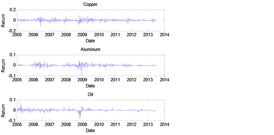
Figure 1. Time series of log-returns of Copper, Aluminum, and Oil. Data source: shanghai futures exchange (http://www.futuresmonthly.com).

Table 1. Kendall rank correlation coefficient matrix for log-returns of Copper, Aluminum and Oila.
aA key attribute of a dependence measure for providing guidance on the form of the Copula is that it should be a pure measure of dependence or scale invariant, and should be unaffected by strictly increasing transformations of the data. Obviously, linear correlation is not scale invariant and is affected by the marginal distributions of the data. Thus, the Kendall rank correlation is used to depict the dependence in this paper.
collapse in price during the period. The detailed statistical descriptions of three return series are presented in Table 2. First, the three returns generally exhibit negative skewness and leptokurtosis (the excess kurtosis is significantly above 0) and reject the null hypothesis of Jarque-Bera test, all which indicates that neither series is unconditional normal. Furthermore, the null hypothesis of ADF (Augmented Dickey-Fuller) unit root test for three log-returns is rejected under level of 1%, which indicates that the three log-returns series are stationary, and thus are appropriate for further analysis. At last, the Lagrange Multiplier test for the presence of the ARCH effect indicates clearly that all log-returns show strong conditional heteroscedasticity, a common feature of financial data. In a nutshell, descriptive statistics show that return series of the three spot commodities possess some intrinsicfeatures, including high kurtosis, negative skewness and time varying volatility. For this reason, GARCH class models should be used to describe the dynamics behaviors of these return series.
A preliminary analysis of autocorrelation and partial autocorrelation function of log-returns and autocorrelation function of squared log-returns of three spot commodity samples, presented in Figure 2, shows that these functions decay slowly to zero as lags increase. The analysis may indicate that there is high order autocorrelation in log-returns and dual long memory in both mean and variance. To address this, the ARFIMA-FIGARCH class models will be effective in modeling these log-returns series.
4.2. Results of Long Memory Tests
Long memory in volatility is an intrinsic empirical feature of any financial variables. The presence of long memory in the volatility of the time series implies that there is nonlinear dependence in the dynamics volatility process, which thus promotes the potential of long-term predictability of the volatility. Testing for long memory property is an essential task since any evidence of long memory in volatility would support the use of long memory
Table 2. Descriptive statistics, ARCH LM test and unit root testsa.
aJ-Band ARCH(10) refer respectively to the empirical statistics of Jarque-Bera test for normality, and Engle LM test for conditional heteroscedasticity. ***Represents statistical significance at the 1% level.
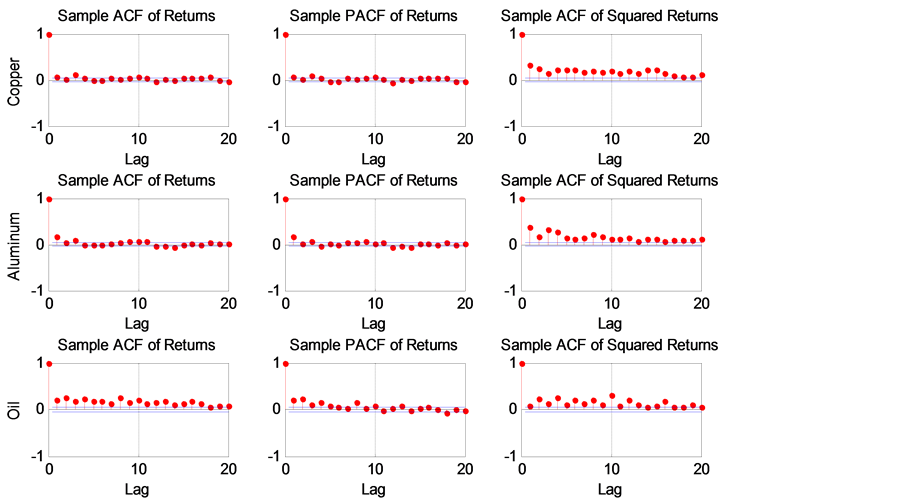
Figure 2. Autocorrelation, partial autocorrelation of log-returns and autocorrelation of squared log-returns.
FIGARCH models rather than GARCH models with short memory.
In this paper, we use three long memory estimation methods. Two semi-parametric methods: 1) the log-peri- odogram regression (GPH) test (Geweke and Porter-Hudak [42] ) and 2) the Gaussian semi-parametric (GSP) test (Robinson [43] ), and one non-parametric methods: 3) the modified Rescaled Statistic (R/S) of Lo [44] .
We apply the three long memory tests to the raw returns and squared returns of the inventories (the latter are frequently used as a proxy for financial volatility, e.g., Arouri et al. [14] ). The results of the tests are documented in Table 3. Panel A of Table 3 shows that Lo’s R/S test statistics support the null hypothesis of short memory in the returns (except the returns of Oil), whereas the statistics indicate that there is long memory behavior in the volatility process.
From Panel B and C of Table 3, we can clearly notice that both GPH and GSP tests do not reject the null hypothesis of no long-range dependence in the three inventory returns (except the returns of Oil). For the squared return series, the results of the both tests provide strong evidence of long memory in volatility. This finding implies that there is long-range dependence in volatility, which will be better modeled by a FIGARCH type model.
Overall, the results suggest the ARFIMA-FIGARCH type models are appropriate for accommodating the long memory feature of the volatility, as far as the modeling and forecasting of commodity return volatility are concerned.
Table 3. Long memory tests resultsa.
aq denotes the optimal value of the truncation parameter. As the problem of choosing the optimal value of q is not yet solved, it might be useful to apply several tests and consider a range of values of q. In this paper, we consider in the empirical part three values of q = 1, q = 5 and q = 10. The critical value of Lo’s modified R/S statistic is 2.098 at the 1% level. Likewise, long memory tests are very sensitive to the selection of bandwidth m for the GPH and GSP tests. Thus, the GPH test is applied with different bandwidths: m = T0.5, m = T0.6 and m = T0.8. For the GSP test, it was estimated for diverse bandwidths: m = T/4, m = T/8 and m = T/16. T is the total number of observations. The associated p-values are reported in brackets.
4.3. The Effects of Long Memory on Modeling and Forecasting Marginal Distribution
4.3.1. The Effects of Long Memory on Estimation Results in Sample
In this subsection, we compare estimates of long memory volatility models, FIGARCH, and short memory counterparts, i.e., GARCH and IGARCH in terms of various in-sample criteria: LL, AIC, SIC and HQ. Tables 4-6 present the results of the estimation of the GARCH class models for the Copper, Aluminum and Oil respectively. For each table, the best model is given in bold face, for it has higher value of LL, lower values of AIC, SIC and HQ. The residuals tests are also carried out to check if the chosen volatility model is the most appropriate. In order to capture skewness and fat-tails, the skewed student t distribution is incorporated into this study. For the Oil, the estimations of the long memory GARCH type models with Skewed student t distribution are not computed, because the regularity and non-negativity conditions are not observed, thus we suppose the standardized residuals
Table 4. Estimation results of long memory FIGARCH and short memory GARCH class models with Skewed-t distribution for Coppera.
aStandard errors are in parentheses (.). v is degree freedom of Skewed t distribution; Log(ξ)denotes the asymmetry parameter of Skewed t distribution. LL is the log-likelihood value. AIC, SC and HQ correspond to the Akaike, Schwarz and Hannan-Quinn criteria, respectively. Values in bracket are the p-values associated with statistical tests. *, ** and *** represent the significance at the 10%, 5% and 1% levels, respectively.
Table 5. Estimation results of long memory FIGARCH and short memory GARCH class models for Aluminum with skewed-t distribution.
Table 6. Estimation results of long memory FIGARCH and short memory GARCH class models for Oil with normal distribution.
follow standard normal distribution. That is why we introduce the EVT to model the tail distribution of standardized residuals.
For Copper, Table 4 shows slight long memory behavior for the raw returns. According to the value of LL, AIC and BIC, ARMA(3,3) is the best model to fit the conditional mean equation. With respect to the estimates of the conditional variances, we first observe that the fractional difference parameter and other estimated parameters via FIGARCH model are significant. Moreover, FIGARCH model outperforms the two short memory counterparts in terms of in-sample criteria. It is worth noting that, the stationary condition of volatility for the standard GARCH(1,1) model is not guaranteed since the sum of the ARCH and GARCH coefficients is more than one (the value is 1.003). According to these findings, we can conclude that, the standard GARCH(1,1) model have similar property to that of IGARCH model, which is not suited for out of sample volatility forecasting, especially long-term forecasting. Hence, the FIGARCH model can best model the long memory behavior for Copper.
The results for Aluminum presented in Table 5 are almost similar to those for Copper. For the conditional mean, we fit the AR(1) process to capture the autocorrelation of returns, in terms of LL, AIC and BIC. When it comes to the conditional variance, the long memory parameter is significant at the 1% level, which indicates the presence of long memory in volatility of Aluminum. Moreover, the stationary condition for the standard GARCH(1,1) model is also not guaranteed since the sum of the ARCH and GARCH coefficients is more than one (the value is 1.303). From the perspective of criteria in-sample, FIGARCH model is preferable to other competing models.
The results for heating oil are finally presented in Table 6. For the conditional mean, we fit the ARFIMA(1,d,1) process to capture the long memory and autocorrelation of oil returns, in terms of LL, AIC and BIC. The long memory parameters both in conditional mean and conditional volatility are all significant at the 1% level, which is consistent with the results of long memory test in Table 3. This finding indicates the presence of dual long memory in heating oil. Moreover, the stationary condition for the standard GARCH(1,1) model is not guaranteed since the sum of the ARCH and GARCH coefficients is more than one. Hence, the FIGARCH model outperforms other two competing models according to various in-sample criteria.
To sum up, the results of tests applied to standardized squared residuals indicated that FIGARCH(1,d,1) with Skewed Student-t distributions (Copper, Aluminum)and normal distribution (Oil) are correctly specified because the hypotheses of no autocorrelation and no remaining ARCH effects cannot be rejected in almost all cases. In addition, even though residual series still depart from normality, the values of J-B statistics are generally much lower than those of the raw returns.
4.3.2. The Effects of Long Memory on Multi-Period Volatility Forecasts
In order to further assess the consequences of the specification and also misspecification of the conditional variance equation, out-of-sample multi-period volatility forecasting experiments were conducted. In particular, risk holding horizon, as the key variable to long-term risk prediction, is actually a dynamically adjusted period in portfolio investment strategy, and it is determined by bank’s risk preference, credit of banks’ counterparts, liquidity of inventory and the overall operation situation of supply chain [45] . As the supply chain finance based on spot trading develops more standardized in the age of big data, the liquidity of inventories will be further improved, and the risk holding horizon will be gradually shortened. Therefore, we set the risk holding horizon as 1 day (daily), 5 days (weekly), 10 days (biweekly), 22 days (monthly) and 66 days (quarterly) to make analysis.
All the models were estimated recursively (iterated approach), with ex ante out of sample forecasts generated for daily to quarterly horizons. Indeed, forecast evaluation is a vital component in any forecasting practice. There- fore, we propose to examine the forecasting ability of the estimated GARCH-class of models by using three standard statistical loss functions, the Mean squared error (MSE), Mean Absolute Error (MAE), Root Mean Squared Error (RMSE) and Theil Inequality Coefficient (TIC) (for more details, see e.g., Aloui et al. [13] , Arouri et al. [14] and Charfeddine [16] ). Also, the competing models can be completely evaluated by the use of different loss functions that has different interpretations. The best forecasting model is the one that minimizes these loss functions computed for multi-period volatility forecasts and the results are presented in the Tables 7-9.
Based on forecasting experiments, some interesting conclusions can then be drawn. Firstly, jointly accounting for long memory is important to volatility forecasting of spot commodity returns, particularly at horizons usually of interest, i.e. the monthly and the quarterly. Accounting for long memory can improve specification of the models of GARCH family in all the cases. Secondly, when the stationary condition is not guaranteed, in particular,
Table 7. Out of sample forecasting analysis for the long memory and short memory models-Copper.
Table 8. Out of sample forecasting analysis for the short memory and long memory models-Aluminum.
for the Aluminum, the sum of the ARCH and GARCH coefficients is 1.303 and the values of MSE, MAE and RMSE are worse than FIGARCH model and IGARCH model, especially in the long term forecasting, i.e. the monthly and quarterly.
Taking account of both in-sample criteria and out-of-sample criteria, the best models to fit three marginal distributions are ARMA(3,3)-FIGARCH(1,d,1)-skewed-t, AR(1)-FIGARCH(1,d,1)-skewed-t and ARFIMA(1,d,1)- FIGARCH(1,d,1)-Gaussian models respectively. The IGARCH(1,1) models come second place, while the GARCH(1,1) models are worst. The corresponding standardized residual series can be obtained through the above best models.
4.4. The Effects of Long Memory on Modeling and Forecasting Marginal Distribution
After using ARFIMA-FIGARCH-EVT models to estimate parameters of marginal distributions of three pledged inventories in the first step, we employ IFM method to estimate Copula parameters in the following. First, as mentioned in Section 3, we transform the standardized residuals into uniform variables by the semi-parametric empirical CDF. Furthermore, we use maximum likelihood estimation to fit the multivariate student’s t Copula function, and obtain estimates of the Copula parameters, including the degrees of freedom and the Kendal rank correlation matrix. The results are presented in Table 10. For comparison, the Kendal rank correlation coefficient matrix for standardized residuals derived from the short memory models, i.e. IGARCH, is also shown in the Table 11.
As shown in the Table 10 and Table 11, compared with the case for IGARCH models, Kendal rank correlation coefficient matrix for standardized residuals via long memory FIGARCH models indicate higher degree of dependence between Copper and Aluminum, and lower degree of dependence among Oil with the other two samples, i.e., Copper and Aluminum. Thus, we can conclude that, the presence of long memory in the mean and volatility affects the dependence structure among the returns of pledged inventories. This finding concurs with that conclusion of De Melo Mendes and Kolev [46] , Boubaker and Sghaier [47] .
Table 9. Out of sample forecasting analysis for the short memory and long memory models-Oil.
Table 10. Kendal rank correlation coefficient matrix for standardized residuals (long memory FIGARCH models) through t-Copula function (degree of freedom: 9.518).
Table 11. Kendal rank correlation coefficient matrix for standardized residuals (IGARCH models) through t-Copula function (degree of freedom: 9.926).
4.5. The Effects of Long Memory on Inventory Portfolio Optimization
According to the model estimation results based on student’s t Copula function, following the process procedures in Subsection 3.3, we simulate the returns of three samples in the future h trading days for 10,000 times1, and then obtain the long-term log-returns in the following trading days due to the additivity of log-returns, namely long-term log-returns matrix of 3 × 10,000 portfolio. Furthermore, we convert the matrix into arithmetic returns matrix. In order to obtain the efficient frontier of portfolio, the stable convergence of arithmetic returns should be guaranteed, and therefore we set the interval of the arithmetic returns as [−100%, 100%]. At last, we obtain the efficient frontier of the inventory portfolio under the optimization framework of Mean-CVaR in different risk windows at confidence level of 99% based on internal models recommended by Basel Accord and China Bank Regulatory Commission.
Figure 3 shows two efficient frontiers based on the long-term risk with long memory in volatility (FIGARCH(1,d,1) models) and without long memory in volatility (IGARCH models). The efficient frontiers offer maximal expected return for some given level of risk and minimal risk for some given level of expected return. In this way, we obtained the optimal portfolios.
According to Figure 3, we obtained two findings. First, as the risk window becomes longer, the discrepancy between the efficient frontiers with long memory in volatility and without long memory in volatility become lager. This result reveals that, for a given expected return level, the persistence of volatility (long memory) masks the real risk level. If we ignore the important salient characteristics, the real risk level will be misestimated, especially in the long-term risk measure, such as monthly and quarterly measure.
Furthermore, for shorter term risk windows (daily to biweekly), as returns get close to zero, the two efficient frontiers are clearly distinct. However, the two efficient frontiers merge gradually as the risk increases, and finally the efficient frontier based on long memory lies above the short memory efficient frontier. From this phenomenon, we can conclude that, if the bank is conservative (i.e., risk averse), the IGARCH models will underes-
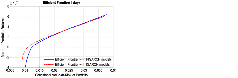
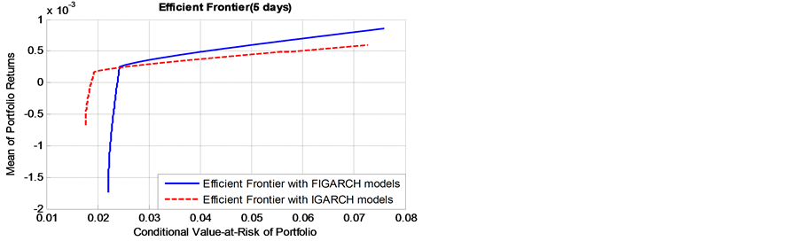
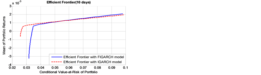
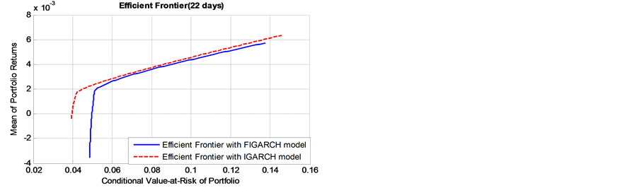
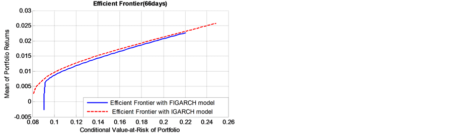
Figure 3. Efficient frontiers for different risk windows in the both cases of with and without long memory.
timate the actual risk level; if the bank is aggressive (i.e., risk lover), the IGARCH models will overestimate the real risk level. In contrast, when it comes to the long-term risk windows (monthly to quarterly), the IGARCH models will underestimate the real risk level, regardless of that the bank is aggressive or conservative.
5. A Sensitive Analysis of Long Memory Parameter d
In this section, we will further investigate the following question: what is the relationship between the degree of long memory of FIGARCH(1,d,1) model and the risk term structure of inventory portfolio? To this end, we first perform a Monte Carlo simulation to generate the simulation data with different long memory parameters.
In order to concentrate on the estimation of conditional variance parameters in data generation process, conditional mean was fixed at zero across all the simulation experiments. Moreover, the standardized residuals are assumed to follow standard normal distribution2. As noted by Baillie et al. [10] , a sufficient condition for non-negativity of the conditional variance for the FIGARCH(1,d,1) model requires ,
,  and
and . Besides, given the long memory and relatively slow decay of a response to a lagged squared innovation, the effect of pre-sample values might have a bigger impact than stationary GARCH process. Thus, truncating at a too low lag may destroy important long-run dependencies. To mitigate the effects, we set the truncation lag at 1000 for all of the simulation and estimation results below. Moreover, in order to avoid start-up problems, we delete the first 2500 realizations of each replication. Taking account of the condition and constraints in the foregoing, the model parameters for different data generation process are shown in Table 12. All simulations are performed for a sample size of T = 5000. Following the above steps, we construct two groups of portfolio: Portfolio A and Portfolio B. Portfolio A consists of four simulation data samples with d = 0.1, 0.3, 0.5, 0.7 respectively, while Portfolio B consists of four simulation data samples with d = 0.2, 0.4, 0.6, 0.8 respectively. This assumption could ensure that the only difference between Portfolio A and B is the long memory parameters, while other parameters,
  and
and  are same.
In the following, we divide the simulation sample size into two parts: the in-sample (4934 observations) and the out-of-sample (66 observations) in each data generation process. Table 13 and Table 14 presents the results of the estimation of the FIGARCH(1,d,1) models for the different DGP, respectively.
As mentioned in the Section 3, following the procedures of hybrid approach above, we obtain the efficient frontiers of two groups of portfolio under the optimization framework of Mean-CVaR for different risk windows. For sake of brevity, the details are not shown in this paper.
As presented in Figure 4, it is found that, as the value of long memory parameter  of simulation data get bigger, the corresponding efficient frontier of portfolio B lies always above that of initial portfolio A, whether the risk holding horizon is short term (daily), or long-term cases(monthly to quarterly). This finding indicates
Table 12. The parameters design of DGP (Data Generation Process) with standard normal distribution innovation.
Table 13. Estimation results (in-sample simulation data) of FIGARCH(1,d,1) model for Portfolio A.
Table 14. Estimation results (in-sample simulation data) of FIGARCH(1,d,1) model for Portfolio B.
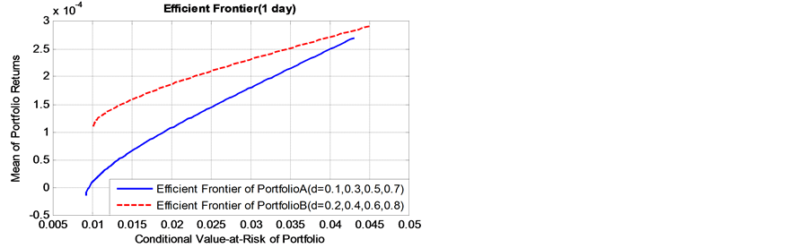
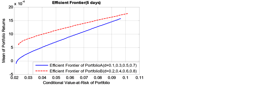
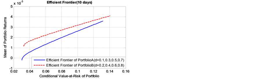
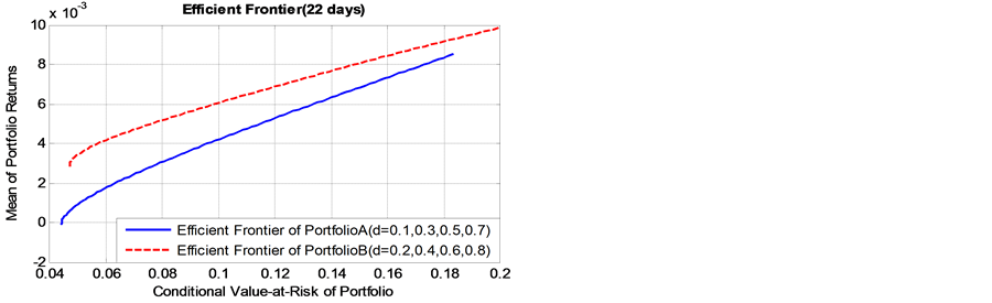
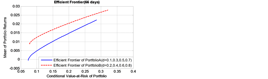
Figure 4. Effect of the long memory degree on efficient frontiers for different risk holding horizon.
that, the portfolio Bpossesses higher expected returns and lower risk level. The conclusion is of significant importance to portfolio selection in supply chain finance, particularly the banks and other participants are risk averse. From the perspective of long memory inconditional volatility, the portfolio which includes spot commodity assets with higher value of long memory parameter will show very promising performance.
6. Conclusions
Long memory in volatility is indispensable in modeling and forecasting multi-period volatility. Different from the portfolio optimization in terms of short-term risk measure for financial assets, we proposed an optimization framework from the perspective of long-term price risk of inventory portfolio with long memory in volatility, and further investigated the impact of long memory on the modeling and forecasting multi-period volatility, the dependence structure and the efficient frontier of inventory portfolio. For this purpose, we established ARFIMA- FIGARCH-EVT type models and multivariate student’s t Copula, and proposed a hybrid approach, combining the iterated approach with the Monte Carlo simulation method, to measure the long-term price risk of inventory portfolio. Moreover, we investigated the relationship between the risk holding horizon (the risk level) and the persistence of long memory via data generation process with different fractional parameter. According to the true data sample (spot Copper, Aluminum and Oil) and simulation data sample, we obtained two main findings: First, for spot commodity with long memory in volatility with parameters , GARCH(d = 0) and IGARCH(d = 1) models will underestimate or overestimate the real risk level of the commodity portfolio, especially for long-term risk window; second, through a sensitive analysis of long memory parameter d that other parameters, i.e.,
  and
and  are fixed, the portfolio being composed of commodities with higher greater value of d, indicates a better efficient frontier for the portfolio.
In conclusion, we provide deep insight into the impact of long memory on price risk measure and portfolio selection for supply chain finance. This paper also leaves possible extensions for future research. One novel extension is to investigate whether the long memory observed in the volatility series of spot commodity is a spurious behavior or not, since some research has been skeptical of the validity of the long memory due to the finding of structural breaks, e.g., Charles et al. [15] and Charfeddine [16] . Secondly, the multivariate Archimedean Copulas and Vine Copulas can be investigated to capture the dependence structure of inventory portfolio. To investigate these issues goes well beyond the scope of the present paper, but represents an interesting avenue for further research.
Acknowledgements
This paper is supported by the National Natural Science Foundation of China (Grant 71003082 & 71273214), China Scholarship Council (No. 201407005086), Education Office of Sichuan Province (SKA13-01) and the Innovation Foundation of Southwest Jiaotong University for PhD Graduates. Acknowledgement goes to Professor Chen Xuebin of Institute for Financial Studies of Fudan University, Professor Zhu Daoli of Antai College of management of Shanghai Jiao Tong University for his suggestion, and Luo Cheng in Shanghai Futures Exchange for his statistical support. The authors would like to thank the anonymous referees for their helpful comments and suggestions, which improved the contents and composition substantially.
Cite this paper
JuanHe,JianWang,XianglinJiang, (2016) The Effects of Long Memory in Price Volatility of Inventories Pledged on Portfolio Optimization of Supply Chain Finance. Journal of Mathematical Finance,06,134-155. doi: 10.4236/jmf.2016.61014
References
- 1. Hofmann, E. and Belin, O. (2011) Supply Chain Finance Solutions: Relevance-Propositions-Market Value. Springer, Berlin.
http://dx.doi.org/10.1007/978-3-642-17566-4 - 2. Pfohl, H.C. and Gomm, M. (2009) Supply Chain Finance: Optimizing Financial Flows in Supply Chains. Logistics Research, 1, 149-161.
http://dx.doi.org/10.1007/s12159-009-0020-y - 3. Wuttke, D.A., Blome, C., Foerstl, K. and Henke, M. (2013) Managing the Innovation Adoption of Supply Chain Finance-Empirical Evidence from Six European Case Studies. Journal of Business Logistics, 34, 148-166.
http://dx.doi.org/10.1111/jbl.12016 - 4. More, D. and Basu, P. (2013) Challenges of Supply Chain Finance: A Detailed Study and a Hierarchical Model Based on the Experiences of an Indian Firm. Business Process Management Journal, 19, 624-647.
http://dx.doi.org/10.1108/BPMJ-09-2012-0093 - 5. Cossin, D., Aunon, N.D. and Gonzales, F. (2003) A Framework for Collateral Risk Control Determination. Working Paper Series 209, European Central Bank, Frankfurt, 1-47.
- 6. Ghysels, E., Valkanov, R.I. and Serrano, A.R. (2009) Multi-Period Forecasts of Volatility: Direct, Iterated, and Mixed-Data Approaches. Proceedings of the EFA 2009 Bergen Meetings, Bergen, 17 February 2009.
http://dx.doi.org/10.2139/ssrn.1344742 - 7. Kinateder, H. and Wagner, N. (2014) Multiple-Period Market Risk Prediction under Long Memory: When VaR Is Higher Than Expected. Journal of Risk Finance, 15, 4-32.
http://dx.doi.org/10.1108/JRF-07-2013-0051 - 8. Hansen, P. and Lunde, A. (2005) A Forecast Comparison of Volatility Models: Does Anything Beat a GARCH(1,1)? Journal of Applied Econometrics, 20, 873-889.
http://dx.doi.org/10.1002/jae.800 - 9. Andersen, T.G. and Bollerslev, T. (1998) Answering the Skeptics: Yes, Standard Volatility Models Do Provide Accurate Forecasts. International Economic Review, 39, 885-905.
http://dx.doi.org/10.2307/2527343 - 10. Baillie, R.T., Bollerslev, T. and Mikkelsen, H.O. (1996) Fractionally Integrated Generalized Autoregressive Conditional Heteroskedasticity. Journal of Econometrics, 74, 3-30.
http://dx.doi.org/10.1016/S0304-4076(95)01749-6 - 11. Elder, J. and Serletis, A. (2008) Long Memory in Energy Futures Prices. Review of Financial Economics, 17, 146-155.
http://dx.doi.org/10.1016/j.rfe.2006.10.002 - 12. Cunado, J., Gil-Alana, L.A. and de-Gracia, F.P. (2010) Persistence in Some Energy Futures Markets. Journal of Futures Market, 30, 490-507.
http://dx.doi.org/10.1002/fut.20426 - 13. Aloui, C. and Mabrouk, S. (2010) Value-at-Risk Estimations of Energy Commodities via Long Memory, Asymmetry and Fat-tailed GARCH Models. Energy Policy, 38, 2326-2339.
http://dx.doi.org/10.1016/j.enpol.2009.12.020 - 14. Arouri, M.E.H., Hammoudeh, S., Lahiani, A. and Nguyen, D.K. (2012) Long Memory and Structural Breaks in Modeling the Return and Volatility Dynamics of Precious Metals. The Quarterly Review of Economics and Finance, 52, 207-218.
http://dx.doi.org/10.1016/j.qref.2012.04.004 - 15. Charles, A. and Darné, O. (2014) Volatility Persistence in Crude Oil Markets. Energy Policy, 65, 729-742.
http://dx.doi.org/10.1016/j.enpol.2013.10.042 - 16. Charfeddine, L. (2014) True or Spurious Long Memory in Volatility: Further Evidence on the Energy Futures Markets. Energy Policy, 71, 76-93.
http://dx.doi.org/10.1016/j.enpol.2014.04.027 - 17. Youssef, M., Belkacem, L. and Mokni, K. (2015) Value-at-Risk Estimation of Energy Commodities: A Long-Memory GARCH-EVT Approach. Energy Economics, 51, 99-110. http://dx.doi.org/10.1016/j.eneco.2015.06.010
- 18. He, J., Jiang, X.L., Wang, J., Zhu, D.L. and Zhen, L. (2012) VaR Methods for the Dynamic Impawn Rate of Steel in Inventory Financing under Autocorrelative Return. European Journal of Operational Research, 223, 106-115.
http://dx.doi.org/10.1016/j.ejor.2012.06.005 - 19. Markowitz, H.M. (1952) Portfolio Selection. Journal of Finance, 7, 77-91.
http://dx.doi.org/10.2307/2975974 - 20. Engle, R.F. (2002) Dynamic Conditional Correlation: A Simple Class of Multivariate Generalized Autoregressive Conditional Heteroskedasticity Models. Journal of Business and Economic Statistics, 20, 339-350.
http://dx.doi.org/10.1198/073500102288618487 - 21. Sklar, A. (1959) Fonctions de répartition à n dimensions etleursmarges. Publications de l’Institut de Statistique de Université de Paris, 8, 229-231.
- 22. Embrechts, P., McNeil, A.J. and Straumann, D. (1999) Correlation: Pitfalls and Alternatives. Risk Magazine, 12, 69-71.
- 23. Jondeau, E. and Rockinger, M. (2006) The Copula-GARCH Model of Conditional Dependencies: An International Stock Market Application. Journal of International Money and Finance, 25, 827-853.
http://dx.doi.org/10.1016/j.jimonfin.2006.04.007 - 24. Fantazzini, D. (2009) The Effects of Misspecified Marginals and Copulas on Computing the Value at risk: A Monte Carlo Study. Computational Statistics and Data Analysis, 53, 2168-2188.
http://dx.doi.org/10.1016/j.csda.2008.02.002 - 25. Wei&beta, G.N.F. (2011) Are Copula-GoF-Tests of Any Practical Use? Empirical Evidence for Stocks, Commodities and FX Futures. The Quarterly Review of Economics and Finance, 51, 173-188.
- 26. Harris, R.D.F. and Mazibas, M. (2013) Dynamic Hedge Fund Portfolio Construction: A Semi-Parametric Approach. Journal of Banking & Finance, 37, 139-149.
http://dx.doi.org/10.1016/j.jbankfin.2012.08.017 - 27. Ignatieva, K. and Trück, S. (2016) Modeling Spot Price Dependence in Australian Electricity Markets with Applications to Risk Management. Computers & Operations Research, 66, 415-433.
http://dx.doi.org/10.1016/j.cor.2015.07.019 - 28. Bollerslev, T. and Mikkelsen, H.O. (1996) Modeling and Pricing Long Memory in Stock Market Volatility. Journal of Econometrics, 73, 151-184.
http://dx.doi.org/10.1016/0304-4076(95)01736-4 - 29. Andersen, T.G., Bollerslev, T., Christoffersen, P.F. and Diebold, F.X. (2006) Volatility and Correlation Forecasting. In: Elliott, G., Granger, C.W.J. and Timmermann, A., Eds., Handbook of Economic Forecasting, North-Holland, Amsterdam, 778-878.
- 30. Artzner, P., Delbaen, F., Eber, J.M. and Heath, D. (1999) Coherent Measures of Risk. Mathematical Finance, 9, 203-228.
http://dx.doi.org/10.1111/1467-9965.00068 - 31. Rockafellar, R.T. and Uryasev, S. (2002) Conditional Value-at-Risk for General Loss Distributions. Journal of Banking & Finance, 26, 1443-1471.
http://dx.doi.org/10.1016/S0378-4266(02)00271-6 - 32. Quaranta, A.G. and Zaffaroni, A. (2008) Robust Optimization of Conditional Value at Risk and Portfolio Selection. Journal of Banking & Finance, 32, 2046-2056.
http://dx.doi.org/10.1016/j.jbankfin.2007.12.025 - 33. Yao, H.X., Li, Z.F. and Lai, Y.Z. (2013) Mean-CVaR Portfolio Selection: A Nonparametric Estimation Framework. Computers & Operations Research, 40, 1014-1022.
http://dx.doi.org/10.1016/j.cor.2012.11.007 - 34. Davidson, J.E. (2004) Moment and Memory Properties of Linear Conditional Heteroscedasticity Models, and a New Model. Journal of Business & Economic Statistics, 22, 16-29.
http://dx.doi.org/10.1198/073500103288619359 - 35. Baillie, R.T. and Morana, C. (2009) Modelling Long Memory and Structural Breaks in Conditional Variances: An Adaptive FIGARCH Approach. Journal of Economic Dynamics and Control, 33, 1577-1592.
http://dx.doi.org/10.1016/j.jedc.2009.02.009 - 36. Lux, T. and Morales-Arias, L. (2013) Relative Forecasting Performance of Volatility Models: Monte Carlo Evidence. Quantitative Finance, 13, 1375-1394.
http://dx.doi.org/10.1080/14697688.2013.795675 - 37. Patton, A. and Sheppard, K. (2009) Optimal Combinations of Realized Volatility Estimators. International Journal of Forecasting, 25, 218-238.
- 38. Gencay, R., Selcuk, F. and Ulugulyagci, A. (2003) High Volatility, Thick Tails and Extreme Value Theory in Value-at-Risk Estimation. Insurance Mathematics and Economics, 33, 337-356.
http://dx.doi.org/10.1016/j.insmatheco.2003.07.004 - 39. McNeil, A.J. and Frey, R. (2000) Estimation of Tail-Related Risk Measures for Heteroscedastic Financial Time Series: An Extreme Value Approach. Journal of Empirical Finance, 7, 271-300.
http://dx.doi.org/10.1016/S0927-5398(00)00012-8 - 40. Chen, X., Fan, Y. and Patton, A.J. (2004) Simple Tests for Models of Dependence between Multiple Financial Time Series, with Applications to US Equity Returns and Exchange Rates. Discussion Paper 483, Financial Markets Group, London School of Economics, London, 1-36.
http://dx.doi.org/10.2139/ssrn.513024 - 41. Patton, A.J. (2006) Estimation of Multivariate Models for Time Series of Possibly Different Lengths. Journal of applied econometrics, 21, 147-173.
http://dx.doi.org/10.1002/jae.865 - 42. Geweke, J. and Porter-Hudark, S. (1983) The Estimation and Application of Long Memory Time Series Models. Journal of Time Series Analysis, 4, 221-238.
http://dx.doi.org/10.1111/j.1467-9892.1983.tb00371.x - 43. Robinson, P.M. (1995) Log-Periodogram Regression of Time Series with Long Range Dependence. The Annals of Statistics, 23, 1048-1072.
http://dx.doi.org/10.1214/aos/1176324636 - 44. Lo, A.W. (1991) Long-Term Memory in Stock Market Prices. Econometrica, 59, 1279-1313.
http://dx.doi.org/10.2307/2938368 - 45. He, J., Wang, J., Jiang, X.L., Chen, X.F. and Chen, L. (2015) The Long-Term Extreme Price Risk Measure of Portfolio in Inventory Financing: An Application to Dynamic Impawn Rate Interval. Complexity, 20, 17-34.
http://dx.doi.org/10.1002/cplx.21516 - 46. De Melo Mendes, B.V. and Kolev, N. (2008) How Long Memory in Volatility Affects True Dependence Structure. International Review of Financial Analysis, 17, 1070-1086.
http://dx.doi.org/10.1016/j.irfa.2007.06.008 - 47. Boubaker, H. and Sghaier, N. (2013) Portfolio Optimization in the Presence of Dependent Financial Returns with Long Memory: A Copula Based Approach. Journal of Banking & Finance, 37, 361-377.
http://dx.doi.org/10.1016/j.jbankfin.2012.09.006
NOTES

1Here we are trading off faster computation time against the accuracy, and select 10,000 simulations in following, which represent a good compromise between accuracy and speed.
2For sake of space, the data generation process with Skewed student innovation is also simulated; the results are not presented in this paper. In fact, the pattern and speed of shocks decay are dominated by ,
,  and d.