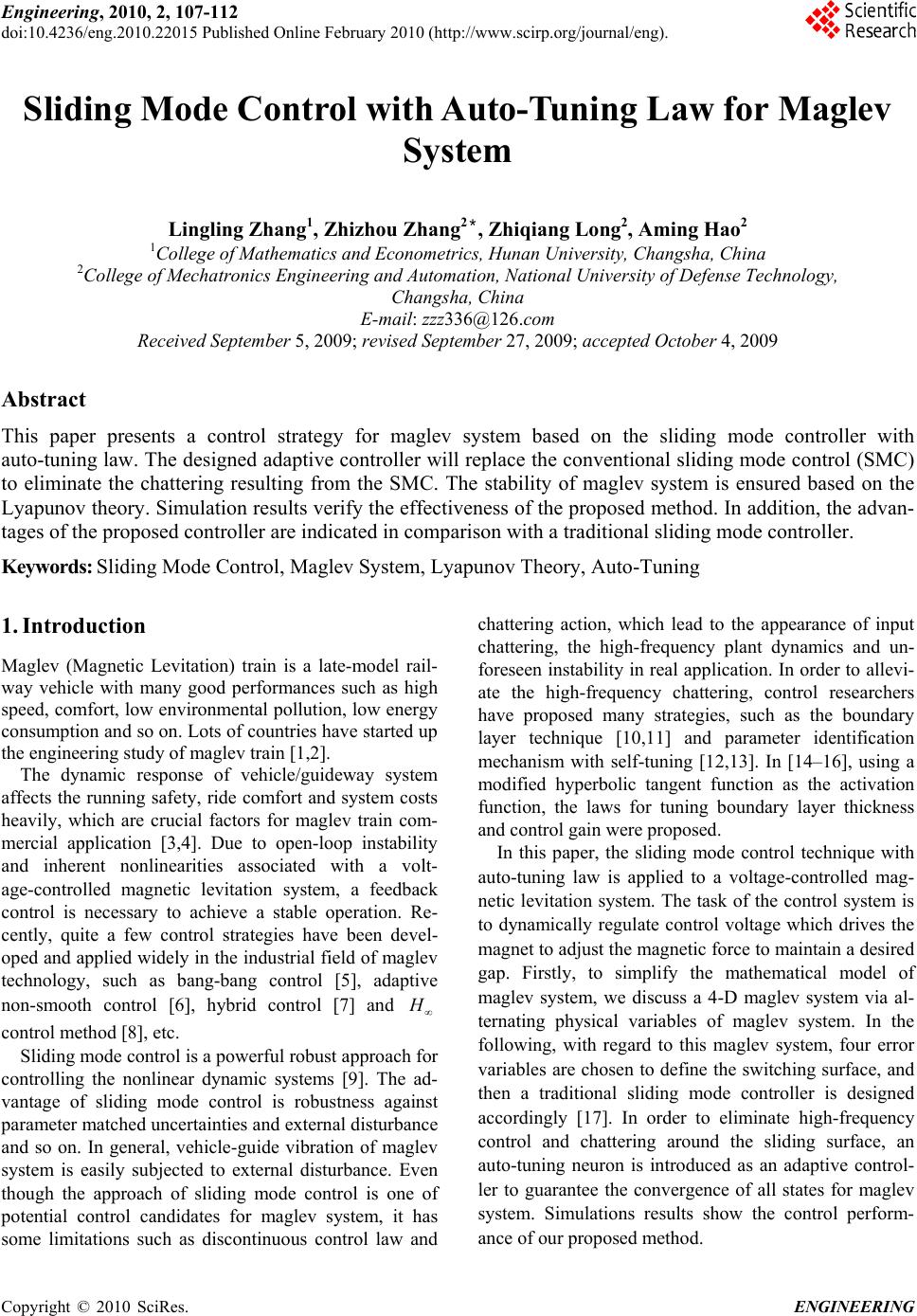Engineering, 2010, 2, 107-112
doi:10.4236/eng.2010.22015 Published Online February 2010 (http://www.scirp.org/journal/eng).
Sliding Mode Control with Auto-Tuning Law for Maglev
System
Lingling Zhang1, Zhizhou Zhang2＊, Zhiqiang Long2, Aming Hao2
1College of Mathematics and Econometrics, Hunan University, Changsha, China
2College of Mechatronics Engineering and Automation, National University of Defense Technology,
Changsha, China
Received September 5, 2009; revised September 27, 2009; accepted October 4, 2009
Abstract
This paper presents a control strategy for maglev system based on the sliding mode controller with
auto-tuning law. The designed adaptive controller will replace the conventional sliding mode control (SMC)
to eliminate the chattering resulting from the SMC. The stability of maglev system is ensured based on the
Lyapunov theory. Simulation results verify the effectiveness of the proposed method. In addition, the advan-
tages of the proposed controller are indicated in comparison with a traditional sliding mode controller.
Keywords: Sliding Mode Control, Maglev System, Lyapunov Theory, Auto-Tuning
1. Introduction
Maglev (Magnetic Levitation) train is a late-model rail-
way vehicle with many good performances such as high
speed, comfort, low environmental pollution, low energy
consumption and so on. Lots of countries have started up
the engineering study of maglev train [1,2].
The dynamic response of vehicle/guideway system
affects the running safety, ride comfort and system costs
heavily, which are crucial factors for maglev train com-
mercial application [3,4]. Due to open-loop instability
and inherent nonlinearities associated with a volt-
age-controlled magnetic levitation system, a feedback
control is necessary to achieve a stable operation. Re-
cently, quite a few control strategies have been devel-
oped and applied widely in the industrial field of maglev
technology, such as bang-bang control [5], adaptive
non-smooth control [6], hybrid control [7] and H
control method [8], etc.
Sliding mode control is a powerful robust approach for
controlling the nonlinear dynamic systems [9]. The ad-
vantage of sliding mode control is robustness against
parameter matched uncertainties and external disturbance
and so on. In general, vehicle-guide vibration of maglev
system is easily subjected to external disturbance. Even
though the approach of sliding mode control is one of
potential control candidates for maglev system, it has
some limitations such as discontinuous control law and
chattering action, which lead to the appearance of input
chattering, the high-frequency plant dynamics and un-
foreseen instability in real application. In order to allevi-
ate the high-frequency chattering, control researchers
have proposed many strategies, such as the boundary
layer technique [10,11] and parameter identification
mechanism with self-tuning [12,13]. In [14–16], using a
modified hyperbolic tangent function as the activation
function, the laws for tuning boundary layer thickness
and control gain were proposed.
In this paper, the sliding mode control technique with
auto-tuning law is applied to a voltage-controlled mag-
netic levitation system. The task of the control system is
to dynamically regulate control voltage which drives the
magnet to adjust the magnetic force to maintain a desired
gap. Firstly, to simplify the mathematical model of
maglev system, we discuss a 4-D maglev system via al-
ternating physical variables of maglev system. In the
following, with regard to this maglev system, four error
variables are chosen to define the switching surface, and
then a traditional sliding mode controller is designed
accordingly [17]. In order to eliminate high-frequency
control and chattering around the sliding surface, an
auto-tuning neuron is introduced as an adaptive control-
ler to guarantee the convergence of all states for maglev
system. Simulations results show the control perform-
ance of our proposed method.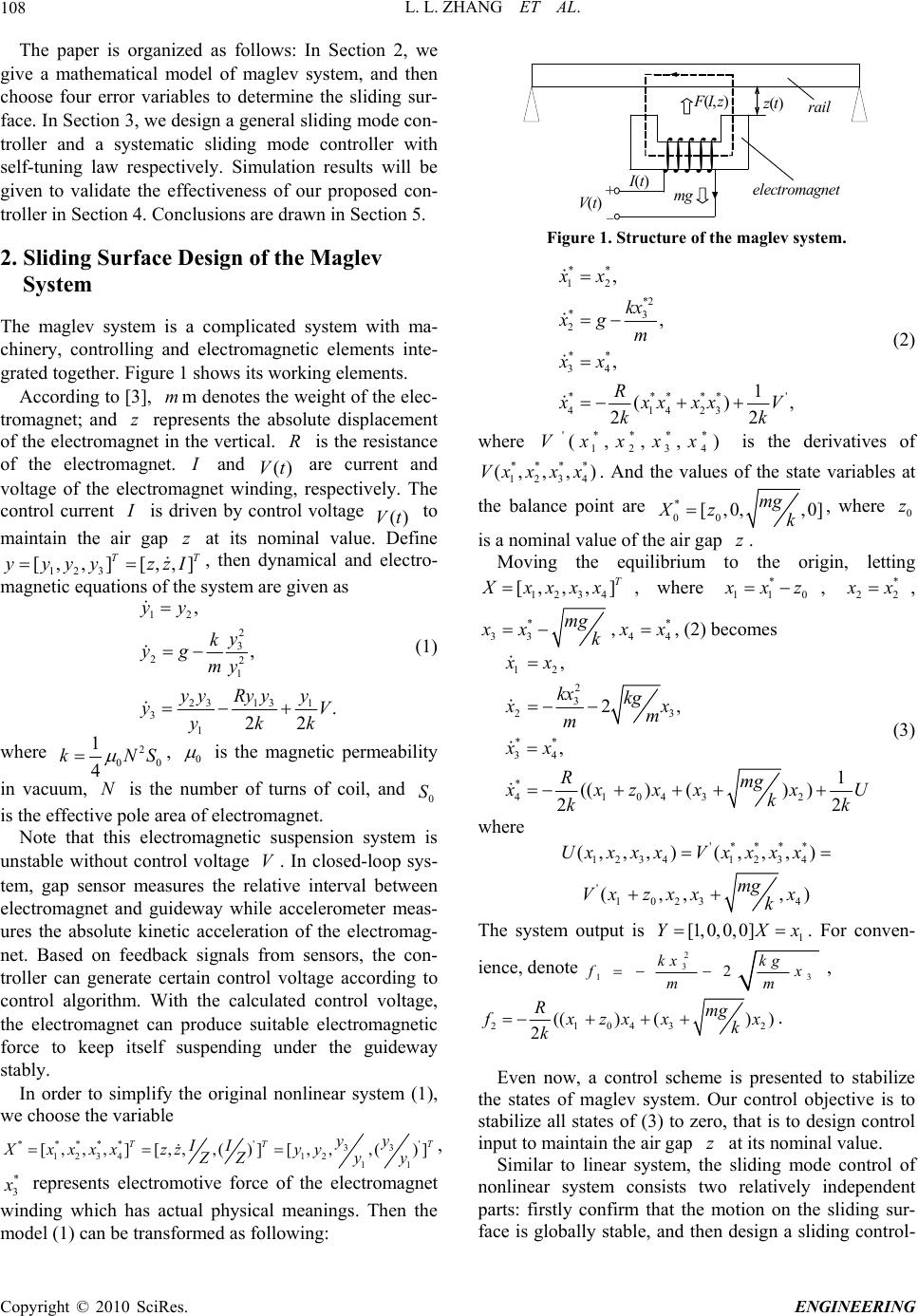

L. L. ZHANG ET AL. 108
The paper is organized as follows: In Section 2, we
give a mathematical model of maglev system, and then
choose four error variables to determine the sliding sur-
face. In Section 3, we design a general sliding mode con-
troller and a systematic sliding mode controller with
self-tuning law respectively. Simulation results will be
given to validate the effectiveness of our proposed con-
troller in Section 4. Conclusions are drawn in Section 5.
2. Sliding Surface Design of the Maglev
System
The maglev system is a complicated system with ma-
chinery, controlling and electromagnetic elements inte-
grated together. Figure 1 shows its working elements.
According to [3], m denotes the weight of the elec-
tromagnet; and represents the absolute displacement
of the electromagnet in the vertical. is the resistance
of the electromagnet.
m
z
R
I
and
()
Vt are current and
voltage of the electromagnet winding, respectively. The
control current
I
is driven by control voltage
()
Vt to
maintain the air gap at its nominal value. Define
123 , then dynamical and electro-
magnetic equations of the system are given as
z
,,zz

[, , ][
T
yyyy]I
T
12
2
3
22
1
2313 1
3
1
,
,
.
22
yy
y k
yg
my
yyRy yy
yV
ykk


 



(1)
where 2
00
1
4
kNS
0
 ,

is the magnetic permeability
in vacuum, is the number of turns of coil, and
is the effective pole area of electromagnet.
N0
S
Note that this electromagnetic suspension system is
unstable without control voltage . In closed-loop sys-
tem, gap sensor measures the relative interval between
electromagnet and guideway while accelerometer meas-
ures the absolute kinetic acceleration of the electromag-
net. Based on feedback signals from sensors, the con-
troller can generate certain control voltage according to
control algorithm. With the calculated control voltage,
the electromagnet can produce suitable electromagnetic
force to keep itself suspending under the guideway
stably.
V
In order to simplify the original nonlinear system (1),
we choose the variable
***** ''
33
123412 11
[,,,] [,,,()][,,,()]
TT
yy
II
Xxxxx zzyy
ZZy y
 


),( zIF )(tz
mg
I(t)
+
-
elect romagnet
rail
V(t)

Figure 1. Structure of the maglev system.
**
12
*2
*3
2
**
34
*****
41423
,
,
,
1
()
22
xx
kx
xgm
xx
R'
,
x
xx xxV
kk



 




(2)
where is the derivatives of
. And the values of the state variables at
the balance point are
'* * * *
1234
(, ,, )Vxxxx
****
1234
,,,)xxx(Vx
*
00
[,Xz0,,0]
mg
k, where
is a nominal value of the air gap .
0
z
z
Moving the equilibrium to the origin, letting
1234
[,, ,]
T
X
xxxx, where *
110
x
xz , *
22
x
x

,
*
33
mg
xx k  ,*
44
x
x

, (2) becomes
12
2
3
23
**
34
*
41043 2
,
2,
,
1
(()() )
22
x
x
kx kg
xx
m
m
xx
Rmg
x
xzx xxU
k
kk

 

 




(3)
where
'****
12341 234
(,,,) (,,,)Uxxxx Vxxxx


'
1 0234
(,, ,
mg
Vx zxxx
k
 )
x
The system output is 1
[1,0,0,0]YX

. For conven-
ience, denote2
3
13
2
kx kg
f
x
mm
 ,
21043
(()() )
2
Rmg
2
f
xzx xx
k
k
 .
T
,
*
3
x
represents electromotive force of the electromagnet
winding which has actual physical meanings. Then the
model (1) can be transformed as following:
Even now, a control scheme is presented to stabilize
the states of maglev system. Our control objective is to
stabilize all states of (3) to zero, that is to design control
input to maintain the air gap at its nominal value.
z
Similar to linear system, the sliding mode control of
nonlinear system consists two relatively independent
parts: firstly confirm that the motion on the sliding sur-
face is globally stable, and then design a sliding control-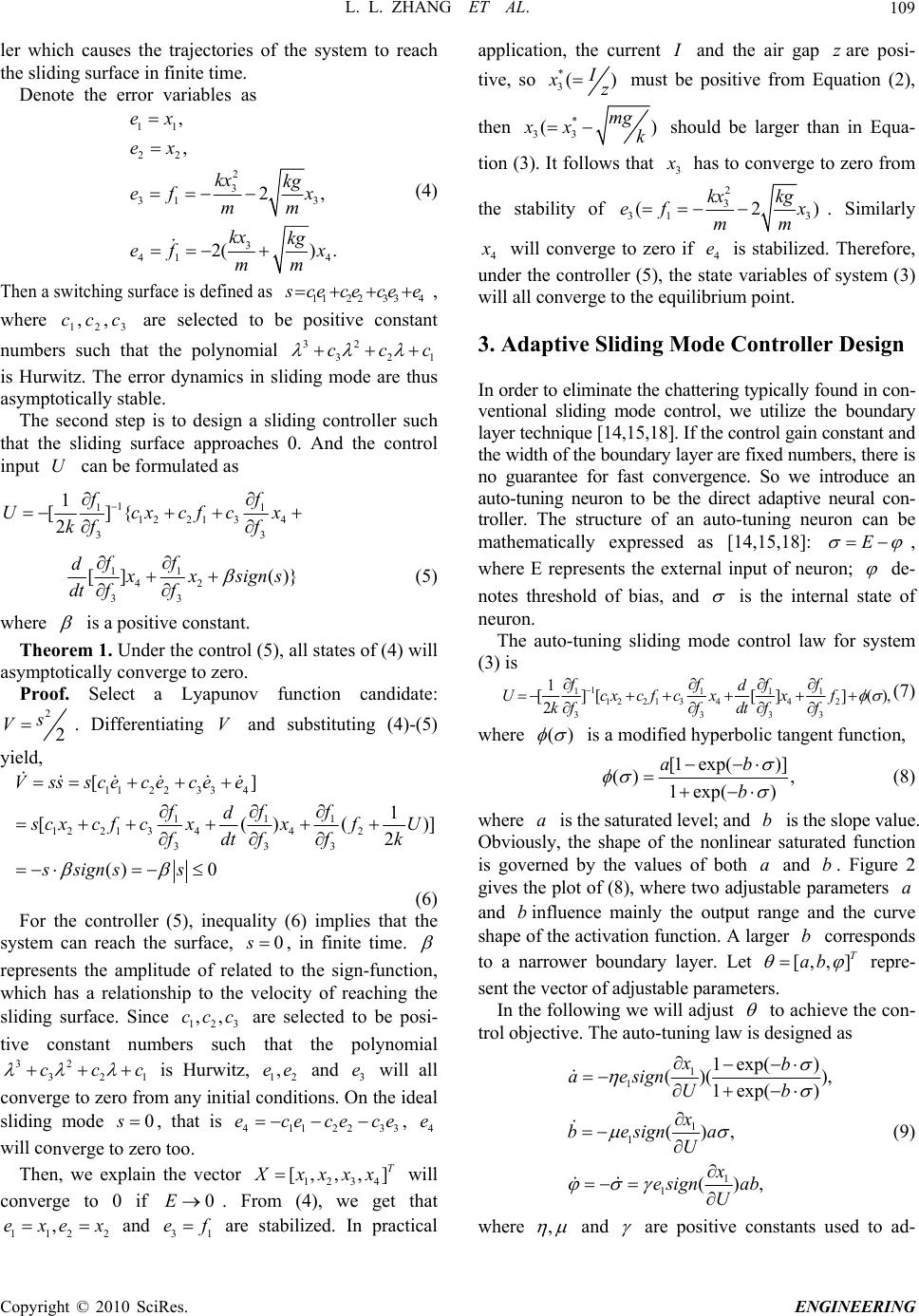

L. L. ZHANG ET AL.109
ler which causes the trajectories of the system to reach
the sliding surface in finite time.
Denote the error variables as
11
22
2
3
31 3
3
41 4
,
,
2
2() .
ex
ex
kx kg
ef x
mm
kx kg
ef x
mm


 
 

,
(4)
Then a switching surface is defined as
112 2334
s
ce cece e
32
32
cc  
,
where are selected to be positive constant
numbers such that the polynomial
is Hurwitz. The error dynamics in sliding mode are thus
asymptotically stable.
123
,,cc c
1
c
The second step is to design a sliding controller such
that the sliding surface approaches 0. And the control
input can be formulated as
U
1 11
1221 34
33
1
[]{
2
ff
Ucxcfc
kf f


 

x
11
42
33
[] ()}
ff
d
x
xsigns
dt ff



 (5)
where

is a positive constant.
Theorem 1. Under the control (5), all states of (4) will
asymptotically converge to zero.
Proof. Select a Lyapunov function candidate:
2
2
s
V. Differentiating V and substituting (4)-(5)
yield,
112 2334
111
1221 3442
333
[]
1
[()()]
2
() 0
Vssscececee
fff
d
s
cxc fcxxfU
fdtffk
ssigns s



 

 

(6)
For the controller (5), inequality (6) implies that the
system can reach the surface, , in finite time.
0s

represents the amplitude of related to the sign-function,
which has a relationship to the velocity of reaching the
sliding surface. Since are selected to be posi-
tive constant numbers such that the polynomial
is Hurwitz, and will all
converge to zero from any initial conditions. On the ideal
sliding mode , that is ,
will converge to zero too.
12
,,ccc
3
1
,ee
41
ec
32
32
cc  
0s
1
c
e
23
e
22
ce
1 3
e c34 e
Then, we explain the vector 1234
[, , , ]
T
X
xxxx will
converge to 0 if . From (4), we get that
and are stabilized. In practical
application, the current
0E
3
ef
112
,exex
21
I
and the air gap are posi-
tive, so
z
*
3()
I
xz  must be positive from Equation (2),
then *
33
(
mg
xx k  ) should be larger than in Equa-
tion (3). It follows that 3
x
has to converge to zero from
the stability of
2
3
31
 3 (2)
kx kg x
mm
 ef . Similarly
4
x
will converge to zero if is stabilized. Therefore,
under the controller (5), the state variables of system (3)
will all converge to the equilibrium point.
4
e
3. Adaptive Sliding Mode Controller Design
In order to eliminate the chattering typically found in con-
ventional sliding mode control, we utilize the boundary
layer technique [14,15,18]. If the control gain constant and
the width of the boundary layer are fixed numbers, there is
no guarantee for fast convergence. So we introduce an
auto-tuning neuron to be the direct adaptive neural con-
troller. The structure of an auto-tuning neuron can be
mathematically expressed as [14,15,18]: E



,
where E represents the external input of neuron;

de-
notes threshold of bias, and

is the internal state of
neuron.
The auto-tuning sliding mode control law for system
(3) is
1
11
4
33
c
f
1
2
3
f
x
1
12 2 4
3
1
[][[]]()
2
fff d
Ucxfx f
kfdt ff
1 3
c,







 (7)
where ()

 is a modified hyperbolic tangent function,
[1
1e
exp(
xp
a)]
() ,
( )
b
b

 

 (8)
where is the saturated level; and is the slope value.
Obviously, the shape of the nonlinear saturated function
is governed by the values of both and b. Figure 2
gives the plot of (8), where two adjustable parameters
and influence mainly the output range and the curve
shape of the activation function. A larger corresponds
to a narrower boundary layer. Let
ab
a
a
b
b
[,,]
T
ab

 repre-
sent the vector of adjustable parameters.
In the following we will adjust

to achieve the con-
trol objective. The auto-tuning law is designed as
1
x
gn
x
ign
U
esig
1
1
1
exp( )
exp( )
,
(),
b
aesUb
be a
n ab
1
1
()(
1
()
x
U
1
i
s
)
,









 


 






 (9)
where ,

and

are positive constants used to ad-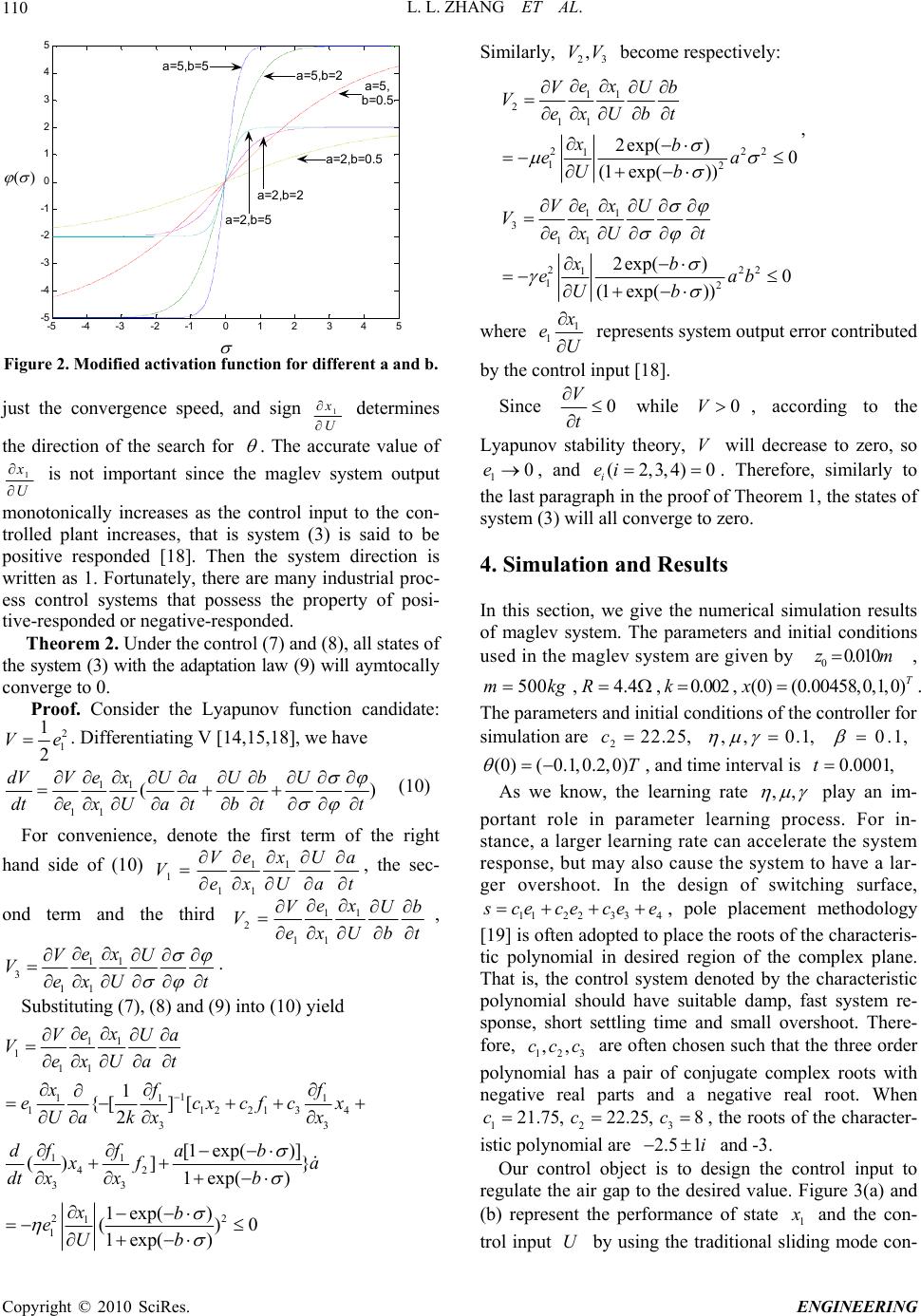

L. L. ZHANG ET AL. 110
-5 -4 -3-2 -10 1 2345
-5
-4
-3
-2
-1
0
1
2
3
4
5
a=5,b=5 a=5,b=2 a=5,
b=0.5
a=2,b=0.5
a=2,b=2
a=2,b=5

()


Figure 2. Modified activation function for different a and b.
just the convergence speed, and sign 1
x
U

 determines
the direction of the search for

. The accurate value of
1
x
U

 is not important since the maglev system output
monotonically increases as the control input to the con-
trolled plant increases, that is system (3) is said to be
positive responded [18]. Then the system direction is
written as 1. Fortunately, there are many industrial proc-
ess control systems that possess the property of posi-
tive-responded or negative-responded.
Theorem 2. Under the control (7) and (8), all states of
the system (3) with the adaptation law (9) will aymtocally
converge to 0.
Proof. Consider the Lyapunov function candidate:
2
1
1
2
Ve. Differentiating V [14,15,18], we have
11
11
(
ex dVVU aUbU
dtexUatbtt )



 

 

(10)
For convenience, denote the first term of the right
hand side of (10) 11
1
11
ex VU
VexUat
a

 
 

, the sec-
ond term and the third 11
2
11
ex VU
VexUbt
 
 
b
,
11
3
11
ex VU
VexU t


 
  

.
Substituting (7), (8) and (9) into (10) yield
11
1
11
1
11 1
11221
33
1
{[] [
2
ex VUa
VexUat
xf f
ecxcfc
Ua kxx



 
 

 
 
34
x
11
42
33
[1 exp()]
() ]}
1exp( )
ff
dab
x
fa
dt xxb


 

 

22
1
1
1exp( )
()
1 exp()
xb
eUb



 

Similarly, become respectively:
23
,VV
11
2
11
22
1
12
2exp()0
(1 exp())
ex VUb
VexUbt
xb
ea
Ub



2




 




,
11
3
11
22 1
12
2exp( )0
(1 exp())
ex
VU
VexU t
xb
ea
Ub
2
b









  




where 1
1
x
eU


represents system output error contributed
by the control input [18].
Since 0
V
t


 while , according to the
Lyapunov stability theory, will decrease to zero, so
, and
0V
V
)0
10e(2,3,4 i
ei

. Therefore, similarly to
the last paragraph in the proof of Theorem 1, the states of
system (3) will all converge to zero.
4. Simulation and Results
In this section, we give the numerical simulation results
of maglev system. The parameters and initial conditions
used in the maglev system are given by00.010zm

,
500mkg

,4.4R

,0. 002k

,.
The parameters and initial conditions of the controller for
(0) ,0)T x(0.00 458,0,1
simulation are 222.25,c

,, 0.1,

  0.1,


(0)( 0.1,0.2,0)T


, and time interval is 0.0001,t
As we know, the learning rate ,,

play an im-
portant role in parameter learning process. For in-
stance, a larger learning rate can accelerate the system
response, but may also cause the system to have a lar-
ger overshoot. In the design of switching surface,
112 23 34
s
ce cecee


123
,,cc c
121.75,c
, pole placement methodology
[19] is often adopted to place the roots of the characteris-
tic polynomial in desired region of the complex plane.
That is, the control system denoted by the characteristic
polynomial should have suitable damp, fast system re-
sponse, short settling time and small overshoot. There-
fore, are often chosen such that the three order
polynomial has a pair of conjugate complex roots with
negative real parts and a negative real root. When

222.25,c

3
c8

, the roots of the character-
istic polynomial are 2.5 1i

 and -3.
Our control object is to design the control input to
regulate the air gap to the desired value. Figure 3(a) and
(b) represent the performance of state 1
x
and the con-
trol input by using the traditional sliding mode con- U
0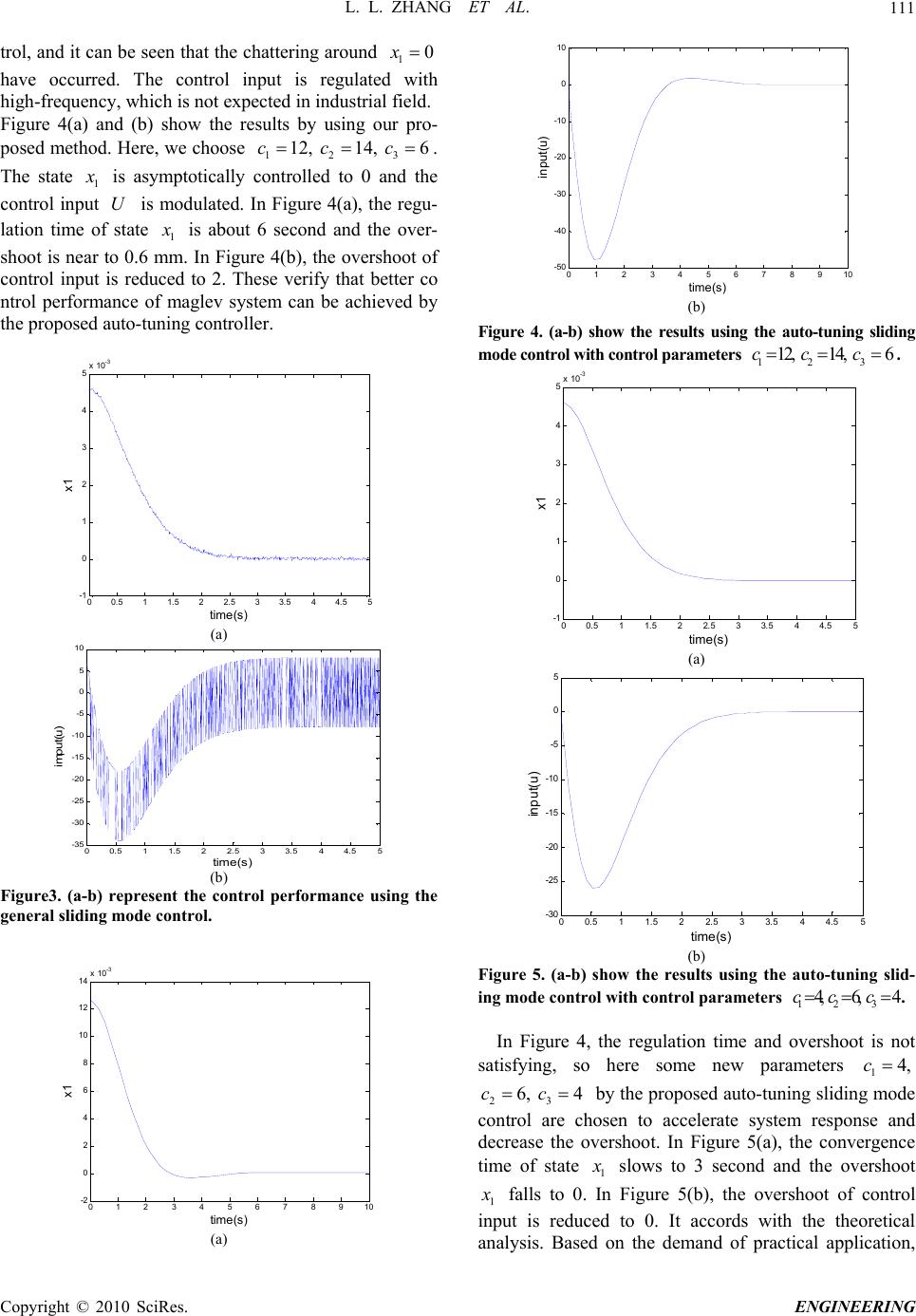

L. L. ZHANG ET AL.111
trol, and it can be seen that the chattering around 10x

have occurred. The control input is regulated with
high-frequency, which is not expected in industrial field.
Figure 4(a) and (b) show the results by using our pro-
posed method. Here, we choose 112,c214,c36c

.
The state 1
x
is asymptotically controlled to 0 and the
control input is modulated. In Figure 4(a), the regu-
lation time of state
U
1
x
is about 6 second and the over-
shoot is near to 0.6 mm. In Figure 4(b), the overshoot of
control input is reduced to 2. These verify that better co
ntrol performance of maglev system can be achieved by
the proposed auto-tuning controller.
00.5 11.5 22.5 33.5 44.5 5
-1
0
1
2
3
4
5x 10
-3
time (s )
x1
(a)
00.5 11.5 22.5 33.5 44.5 5
-35
-30
-25
-20
-15
-10
-5
0
5
10
time
(
s
)
imput(u)
(b)
Figure3. (a-b) represent the control performance using the
general sliding mode control.
0 1 23 45 6 78 910
-2
0
2
4
6
8
10
12
14 x 10
-3
time(s)
x1
(a)
012345678910
-50
-40
-30
-20
-10
0
10
time (s )
input(u)
(b)
Figure 4. (a-b) show the results using the auto-tuning sliding
mode control with control parameters 112,c214,c36c

.
00.5 11.5 22.5 33.5 44.5 5
-1
0
1
2
3
4
5x 10
-3
tim e(s)
x1
(a)
00.5 11.5 22.5 33.5 44.5 5
-30
-25
-20
-15
-10
-5
0
5
tim e(s)
input(u)
(b)
Figure 5. (a-b) show the results using the auto-tuning slid-
ing mode control with control parameters 14,c26,c

34c

.
In Figure 4, the regulation time and overshoot is not
satisfying, so here some new parameters 14,c

26,c

34c

by the proposed auto-tuning sliding mode
control are chosen to accelerate system response and
decrease the overshoot. In Figure 5(a), the convergence
time of state 1
x
slows to 3 second and the overshoot
1
x
falls to 0. In Figure 5(b), the overshoot of control
input is reduced to 0. It accords with the theoretical
analysis. Based on the demand of practical application,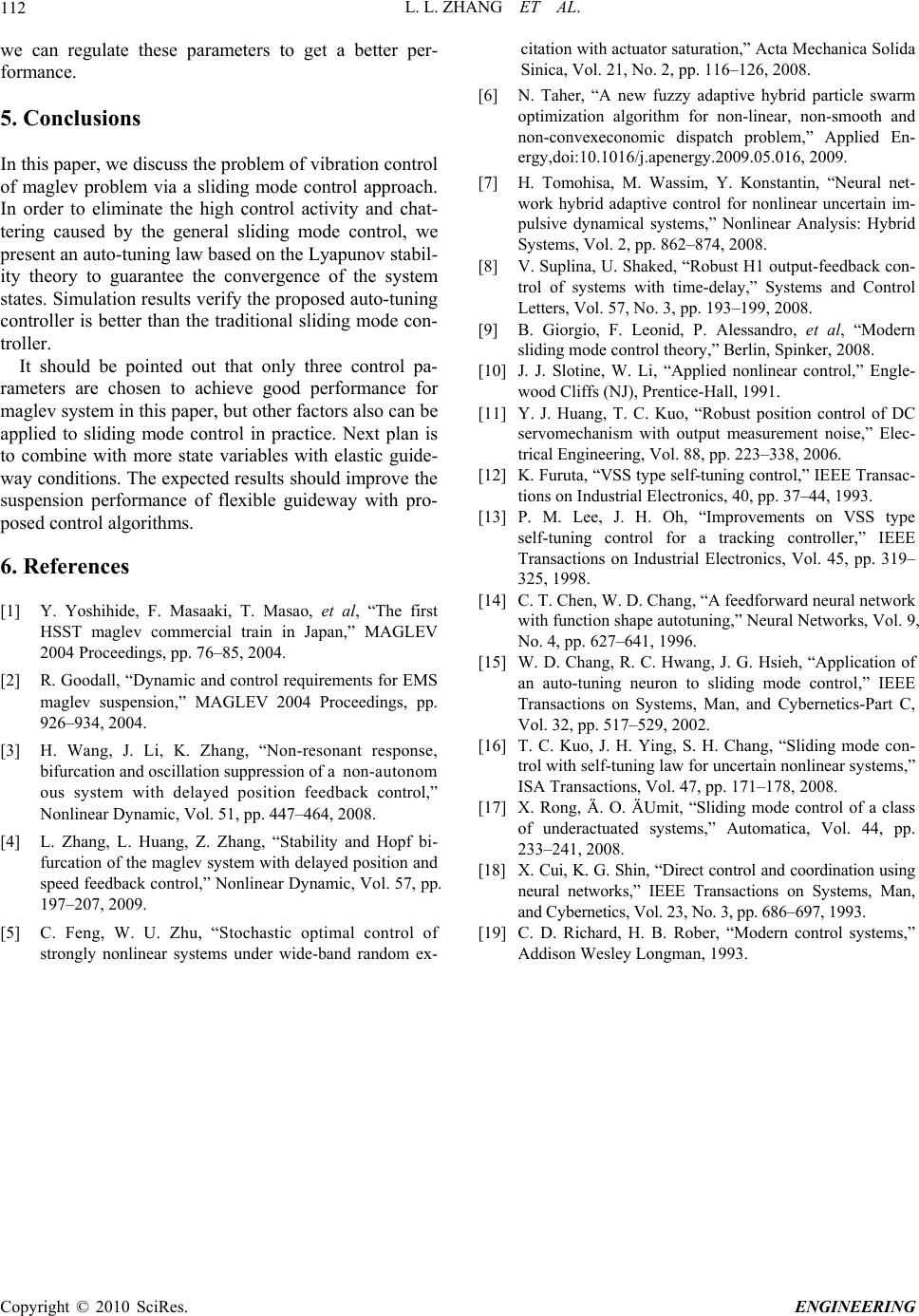

L. L. ZHANG ET AL. 112
we can regulate these parameters to get a better per-
formance.
5. Conclusions
In this paper, we discuss the problem of vibration control
of maglev problem via a sliding mode control approach.
In order to eliminate the high control activity and chat-
tering caused by the general sliding mode control, we
present an auto-tuning law based on the Lyapunov stabil-
ity theory to guarantee the convergence of the system
states. Simulation results verify the proposed auto-tuning
controller is better than the traditional sliding mode con-
troller.
It should be pointed out that only three control pa-
rameters are chosen to achieve good performance for
maglev system in this paper, but other factors also can be
applied to sliding mode control in practice. Next plan is
to combine with more state variables with elastic guide-
way conditions. The expected results should improve the
suspension performance of flexible guideway with pro-
posed control algorithms.
6
. References
[1] Y. Yoshihide, F. Masaaki, T. Masao, et al, “The first
HSST maglev commercial train in Japan,” MAGLEV
2004 Proceedings, pp. 76–85, 2004.
[2] R. Goodall, “Dynamic and control requirements for EMS
maglev suspension,” MAGLEV 2004 Proceedings, pp.
926–934, 2004.
[3] H. Wang, J. Li, K. Zhang, “Non-resonant response,
bifurcation and oscillation suppression of anon-autonom
ous system with delayed position feedback control,”
Nonlinear Dynamic, Vol. 51, pp. 447–464, 2008.
[4] L. Zhang, L. Huang, Z. Zhang, “Stability and Hopf bi-
furcation of the maglev system with delayed position and
speed feedback control,” Nonlinear Dynamic, Vol. 57, pp.
197–207, 2009.
[5] C. Feng, W. U. Zhu, “Stochastic optimal control of
strongly nonlinear systems under wide-band random ex-
citation with actuator saturation,” Acta Mechanica Solida
Sinica, Vol. 21, No. 2, pp. 116–126, 2008.
[6] N. Taher, “A new fuzzy adaptive hybrid particle swarm
optimization algorithm for non-linear, non-smooth and
non-convexeconomic dispatch problem,” Applied En-
ergy,doi:10.1016/j.apenergy.2009.05.016, 2009.
[7] H. Tomohisa, M. Wassim, Y. Konstantin, “Neural net-
work hybrid adaptive control for nonlinear uncertain im-
pulsive dynamical systems,” Nonlinear Analysis: Hybrid
Systems, Vol. 2, pp. 862–874, 2008.
[8] V. Suplina, U. Shaked, “Robust H1 output-feedback con-
trol of systems with time-delay,” Systems and Control
Letters, Vol. 57, No. 3, pp. 193–199, 2008.
[9] B. Giorgio, F. Leonid, P. Alessandro, et al, “Modern
sliding mode control theory,” Berlin, Spinker, 2008.
[10] J. J. Slotine, W. Li, “Applied nonlinear control,” Engle-
wood Cliffs (NJ), Prentice-Hall, 1991.
[11] Y. J. Huang, T. C. Kuo, “Robust position control of DC
servomechanism with output measurement noise,” Elec-
trical Engineering, Vol. 88, pp. 223–338, 2006.
[12] K. Furuta, “VSS type self-tuning control,” IEEE Transac-
tions on Industrial Electronics, 40, pp. 37–44, 1993.
[13] P. M. Lee, J. H. Oh, “Improvements on VSS type
self-tuning control for a tracking controller,” IEEE
Transactions on Industrial Electronics, Vol. 45, pp. 319–
325, 1998.
[14] C. T. Chen, W. D. Chang, “A feedforward neural network
with function shape autotuning,” Neural Networks, Vol. 9,
No. 4, pp. 627–641, 1996.
[15] W. D. Chang, R. C. Hwang, J. G. Hsieh, “Application of
an auto-tuning neuron to sliding mode control,” IEEE
Transactions on Systems, Man, and Cybernetics-Part C,
Vol. 32, pp. 517–529, 2002.
[16] T. C. Kuo, J. H. Ying, S. H. Chang, “Sliding mode con-
trol with self-tuning law for uncertain nonlinear systems,”
ISA Transactions, Vol. 47, pp. 171–178, 2008.
[17] X. Rong, Ä. O. ÄUmit, “Sliding mode control of a class
of underactuated systems,” Automatica, Vol. 44, pp.
233–241, 2008.
[18] X. Cui, K. G. Shin, “Direct control and coordination using
neural networks,” IEEE Transactions on Systems, Man,
and Cybernetics, Vol. 23, No. 3, pp. 686–697, 1993.
[19] C. D. Richard, H. B. Rober, “Modern control systems,”
Addison Wesley Longman, 1993.