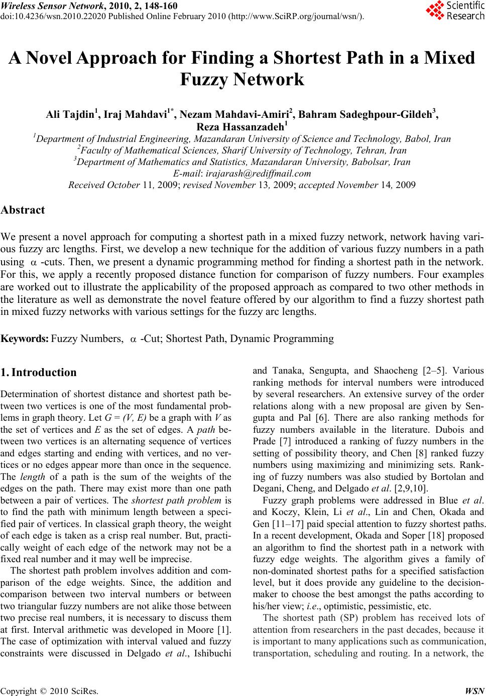Wireless Sensor Network, 2010, 2, 148-160
doi:10.4236/wsn.2010.22020 Published Online February 2010 (http://www.SciRP.org/journal/wsn/).
A Novel Approach for Finding a Shortest Path in a Mixed
Fuzzy Network
Ali Tajdin1, Iraj Mahdavi1*, Nezam Mahdavi-Amiri2, Bahram Sadeghpour-Gildeh3,
Reza Hassanzadeh1
1Department of Industrial Engineering, Mazandaran University of Science and Technology, Babol, Iran
2Faculty of Mathematical Sciences, Sharif University of Technology, Tehran, Iran
3Department of Mathematics and Statistics, Mazandaran University, Babolsar, Iran
Received October 11, 2009; revised November 13, 2009; accepted November 14, 2009
Abstract
We present a novel approach for computing a shortest path in a mixed fuzzy network, network having vari-
ous fuzzy arc lengths. First, we develop a new technique for the addition of various fuzzy numbers in a path
using
α
-cuts. Then, we present a dynamic programming method for finding a shortest path in the network.
For this, we apply a recently proposed distance function for comparison of fuzzy numbers. Four examples
are worked out to illustrate the applicability of the proposed approach as compared to two other methods in
the literature as well as demonstrate the novel feature offered by our algorithm to find a fuzzy shortest path
in mixed fuzzy networks with various settings for the fuzzy arc lengths.
Keywords: Fuzzy Numbers,
α
-Cut; Shortest Path, Dynamic Programming
1. Introduction
Determination of shortest distance and shortest path be-
tween two vertices is one of the most fundamental prob-
lems in graph theory. Let G = (V, E) be a graph with V as
the set of vertices and E as the set of edges. A path be-
tween two vertices is an alternating sequence of vertices
and edges starting and ending with vertices, and no ver-
tices or no edges appear more than once in the sequence.
The length of a path is the sum of the weights of the
edges on the path. There may exist more than one path
between a pair of vertices. The shortest path problem is
to find the path with minimum length between a speci-
fied pair of vertices. In classical graph theory, the weight
of each edge is taken as a crisp real number. But, practi-
cally weight of each edge of the network may not be a
fixed real number and it may well be imprecise.
The shortest path problem involves addition and com-
parison of the edge weights. Since, the addition and
comparison between two interval numbers or between
two triangular fuzzy numbers are not alike those between
two precise real numbers, it is necessary to discuss them
at first. Interval arithmetic was developed in Moore [1].
The case of optimization with interval valued and fuzzy
constraints were discussed in Delgado et al., Ishibuchi
and Tanaka, Sengupta, and Shaocheng [2–5]. Various
ranking methods for interval numbers were introduced
by several researchers. An extensive survey of the order
relations along with a new proposal are given by Sen-
gupta and Pal [6]. There are also ranking methods for
fuzzy numbers available in the literature. Dubois and
Prade [7] introduced a ranking of fuzzy numbers in the
setting of possibility theory, and Chen [8] ranked fuzzy
numbers using maximizing and minimizing sets. Rank-
ing of fuzzy numbers was also studied by Bortolan and
Degani, Cheng, and Delgado et al. [2,9,10].
Fuzzy graph problems were addressed in Blue et al.
and Koczy, Klein, Li et al., Lin and Chen, Okada and
Gen [11–17] paid special attention to fuzzy shortest paths.
In a recent development, Okada and Soper [18] proposed
an algorithm to find the shortest path in a network with
fuzzy edge weights. The algorithm gives a family of
non-dominated shortest paths for a specified satisfaction
level, but it does provide any guideline to the decision-
maker to choose the best amongst the paths according to
his/her view; i.e., optimistic, pessimistic, etc.
The shortest path (SP) problem has received lots of
attention from researchers in the past decades, because it
is important to many applications such as communication,
transportation, scheduling and routing. In a network, the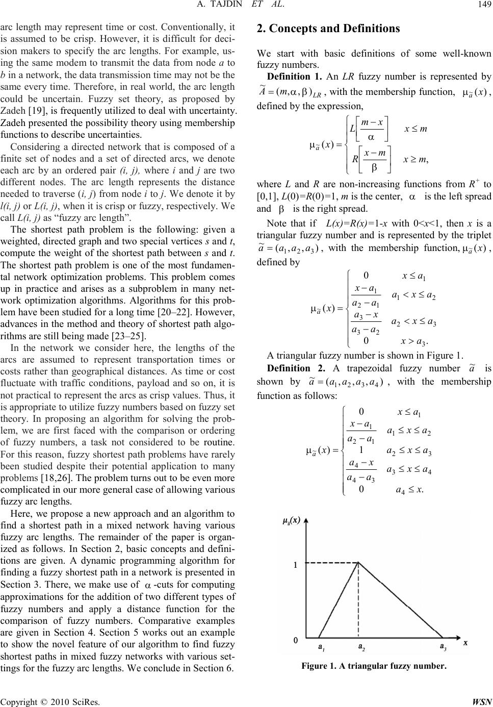

A. TAJDIN ET AL. 149
arc length may represent time or cost. Conventionally, it
is assumed to be crisp. However, it is difficult for deci-
sion makers to specify the arc lengths. For example, us-
ing the same modem to transmit the data from node a to
b in a network, the data transmission time may not be the
same every time. Therefore, in real world, the arc length
could be uncertain. Fuzzy set theory, as proposed by
Zadeh [19], is frequently utilized to deal with uncertainty.
Zadeh presented the possibility theory using membership
functions to describe uncertainties.
Considering a directed network that is composed of a
finite set of nodes and a set of directed arcs, we denote
each arc by an ordered pair (i, j), where i and j are two
different nodes. The arc length represents the distance
needed to traverse (i, j) from node i to j. We denote it by
l(i, j) or L(i, j), when it is crisp or fuzzy, respectively. We
call L(i, j) as “fuzzy arc length”.
The shortest path problem is the following: given a
weighted, directed graph and two special vertices s and t,
compute the weight of the shortest path between s and t.
The shortest path problem is one of the most fundamen-
tal network optimization problems. This problem comes
up in practice and arises as a subproblem in many net-
work optimization algorithms. Algorithms for this prob-
lem have been studied for a long time [20–22]. However,
advances in the method and theory of shortest path algo-
rithms are still being made [23–25].
In the network we consider here, the lengths of the
arcs are assumed to represent transportation times or
costs rather than geographical distances. As time or cost
fluctuate with traffic conditions, payload and so on, it is
not practical to represent the arcs as crisp values. Thus, it
is appropriate to utilize fuzzy numbers based on fuzzy set
theory. In proposing an algorithm for solving the prob-
lem, we are first faced with the comparison or ordering
of fuzzy numbers, a task not considered to be routine .
For this reason, fuzzy shortest path problems have rarely
been studied despite their potential application to many
problems [18,26]. The problem turns out to be even more
complicated in our more general case of allowing various
fuzzy arc lengths.
Here, we propose a new approach and an algorithm to
find a shortest path in a mixed network having various
fuzzy arc lengths. The remainder of the paper is organ-
ized as follows. In Section 2, basic concepts and defini-
tions are given. A dynamic programming algorithm for
finding a fuzzy shortest path in a network is presented in
Section 3. There, we make use of
α
-cuts for computing
approximations for the addition of two different types of
fuzzy numbers and apply a distance function for the
comparison of fuzzy numbers. Comparative examples
are given in Section 4. Section 5 works out an example
to show the novel feature of our algorithm to find fuzzy
shortest paths in mixed fuzzy networks with various set-
tings for the fuzzy arc lengths. We conclude in Section 6.
2. Concepts and Definitions
We start with basic definitions of some well-known
fuzzy numbers.
Definition 1. An LR fuzzy number is represented by
LR
mA ),,(
~
βα=, with the membership function, )(
~x
a
µ,
defined by the expression,







≥





−
≤





−
=
,
)(
~
mx
mx
R
mx
xm
L
x
a
β
α
µ
where L and R are non-increasing functions from R+ to
[0,1], L(0)=R(0)=1, m is the center,
α
is the left spread
and
β
is the right spread.
Note that if L(x)=R(x)=1-x with 0<x<1, then x is a
triangular fuzzy number and is represented by the triplet
),,(
~
321aaaa =, with the membership function, )(
~x
a
µ,
defined by









>
≤<
−
−
≤<
−
−≤
=
.0
0
)(
3
32
23
3
21
12
1
1
~
ax
axa
aa
xa
axa
aa
ax ax
x
a
µ
A triangular fuzzy number is shown in Figure 1.
Definition 2. A trapezoidal fuzzy number a
~
is
shown by ),,,(
~
4321 aaaaa =, with the membership
function as follows:











≤
≤≤
−
−≤≤
≤≤
−
−
≤
=
.0
1
0
)(
4
43
34
4
32
21
12
1
1
~
xa
axa
aa
xaaxa
axa
aa
ax ax
x
a
µ
Figure 1. A triangular fuzzy number.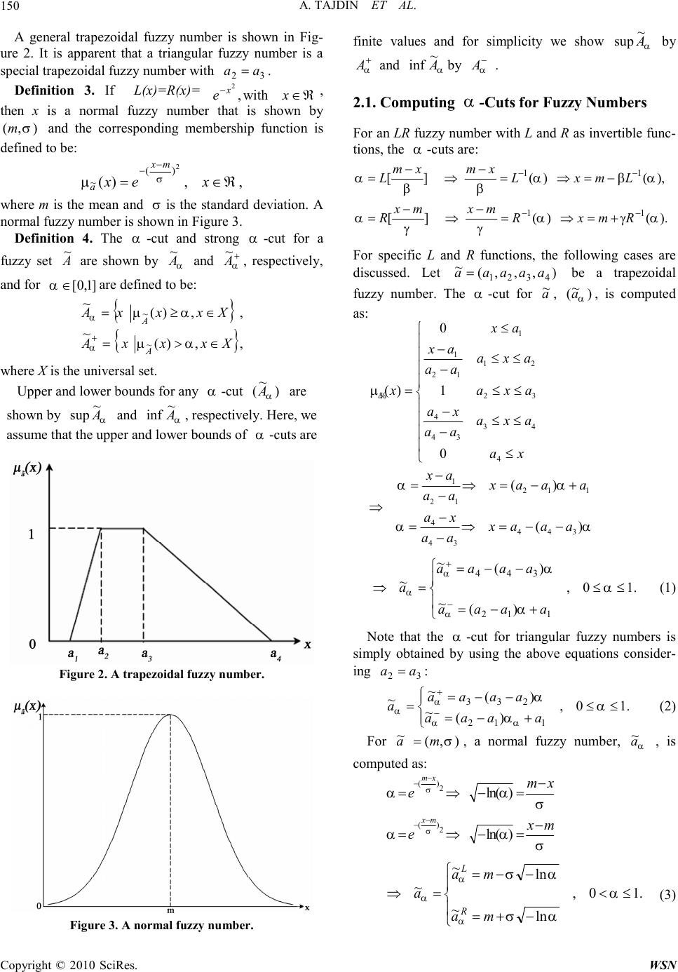

A. TAJDIN ET AL. 150
A general trapezoidal fuzzy number is shown in Fig-
ure 2. It is apparent that a triangular fuzzy number is a
special trapezoidal fuzzy number with 32 aa=.
Definition 3. If L(x)=R(x)=
ℜ
∈
−
x
e
x
with
,
2,
then x is a normal fuzzy number that is shown by
),(σm and the corresponding membership function is
defined to be:
,,)( 2
)(
~ℜ∈=
−
−xex
mx
aσ
µ
where m is the mean and
σ
is the standard deviation. A
normal fuzzy number is shown in Figure 3.
Definition 4. The
α
-cut and strong
α
-cut for a
fuzzy set A
~
are shown by α A
~
and +
α
A
~
, respectively,
and for ]1,0[
∈
α
are defined to be:
{
}
,,)(
~
~XxxxA A∈≥= αµ
α
{
}
,,)(
~
~XxxxA A∈>=
+αµ
α
where X is the universal set.
Upper and lower bounds for any
α
-cut )
~
(α A are
shown by α A
~
sup and α A
~
inf , respectively. Here, we
assume that the upper and lower bounds of
α
-cuts are
Figure 2. A trapezoidal fuzzy number.
Figure 3. A normal fuzzy number.
finite values and for simplicity we show α A
~
sup by
+
α
Aand α A
~
inf by
−
α
A
.
2.1. Computing
α
-Cuts for Fuzzy Numbers
For an LR fuzzy number with L and R as invertible func-
tions, the
α
-cuts are:
).()(][
),()(][
11
11
αγα
γγ
α
αβα
ββ
α
−−
−−
+=⇒=
−
⇒
−
=
−=⇒=
−
⇒
−
=
RmxR
mxmx
R
LmxL
x
m
x
m
L
For specific L and R functions, the following cases are
discussed. Let ),,,(
~
4321 aaaaa = be a trapezoidal
fuzzy number. The
α
-cut for a
~
, )
~
(α a, is computed
as: 1
112
21
23
434
43
4
1
211
21
4443
43
0
()1
0
()
()
a
xa
xa axa
aa
xaxa
axaxa
aa
ax
xa
xaaa
aa
ax xaaa
aa
µ
αα
αα
≤

−
≤≤
−

=≤≤

−
≤≤
−

≤

−
=⇒=−+
−
⇒−
=⇒=−−
−
%





≤≤
+−=
−−=
=⇒
−
+
.10,
)(
~
)(
~
~
112
344 α
α
α
α
α
α
aaaa
aaaa
a (1)
Note that the
α
-cut for triangular fuzzy numbers is
simply obtained by using the above equations consider-
ing 32 aa =:




≤≤
+−=
−−=
=−
+.10,
)(
~)(
~
~
112
233 α
α
α
αα
α
αaaaa
aaaa
a (2)
For ),(
~
σma =, a normal fuzzy number, α a
~
, is
computed as:
()
2
()
2
ln()
ln()
mx
xm
mx
e
xm
e
σ
σ
αα
σ
αα
σ
−
−
−
−
−
=⇒−=
−
=⇒−=
.10,
ln
~
ln
~
~





≤<
−+=
−−=
=⇒ α
ασ
ασ
α
α
α
ma
ma
a
R
L
(3)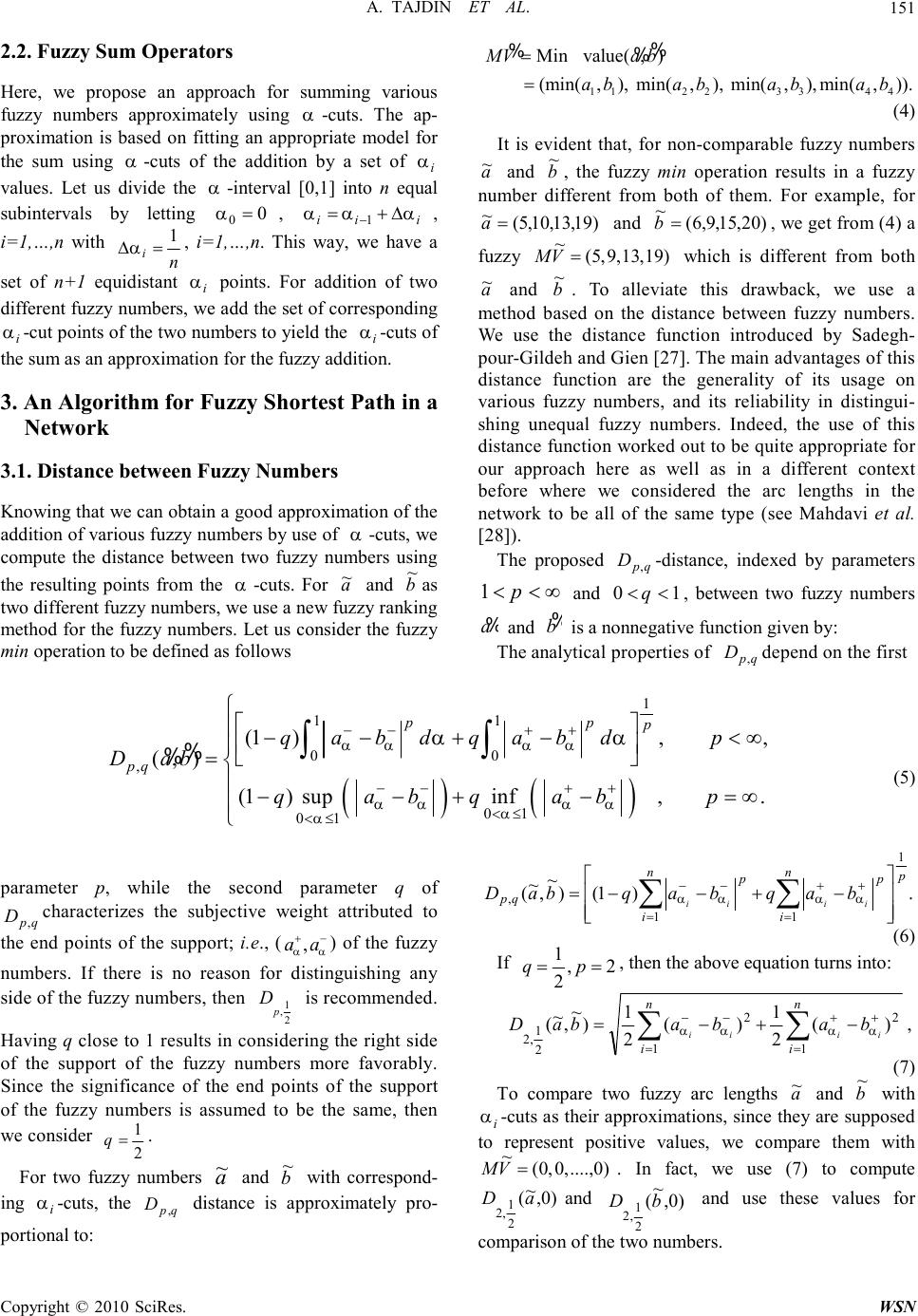

A. TAJDIN ET AL. 151
2.2. Fuzzy Sum Operators
Here, we propose an approach for summing various
fuzzy numbers approximately using
α
-cuts. The ap-
proximation is based on fitting an appropriate model for
the sum using
α
-cuts of the addition by a set of i α
values. Let us divide the
α
-interval [0,1] into n equal
subintervals by letting 0
0=α, iii ααα ∆+= −1,
i=1,…,n with
n
i
1
=∆α, i=1,…,n. This way, we have a
set of n+1 equidistant i α points. For addition of two
different fuzzy numbers, we add the set of corresponding
i
α-cut points of the two numbers to yield the i α-cuts of
the sum as an approximation for the fuzzy addition.
3. An Algorithm for Fuzzy Shortest Path in a
Network
3.1. Distance between Fuzzy Numbers
Knowing that we can obtain a good approximation of the
addition of various fuzzy numbers by use of
α
-cuts, we
compute the distance between two fuzzy numbers using
the resulting points from the
α
-cuts. For a
~
and b
~
as
two different fuzzy numbers, we use a new fuzzy ranking
method for the fuzzy numbers. Let us consider the fuzzy
min operation to be defined as follows
Min
MV =
%
value(,)
ab
%
%
11
(min(,),
ab
=22
min(,),
ab
3344
min(,),min(,)).
abab
(4)
It is evident that, for non-comparable fuzzy numbers
a
~
and b
~
, the fuzzy min operation results in a fuzzy
number different from both of them. For example, for
)19,13,10,5(
~
=a and )20,15,9,6(
~
=b, we get from (4) a
fuzzy )19,13,9,5(
~
=VM which is different from both
a
~
and b
~
. To alleviate this drawback, we use a
method based on the distance between fuzzy numbers.
We use the distance function introduced by Sadegh-
pour-Gildeh and Gien [27]. The main advantages of this
distance function are the generality of its usage on
various fuzzy numbers, and its reliability in distingui-
shing unequal fuzzy numbers. Indeed, the use of this
distance function worked out to be quite appropriate for
our approach here as well as in a different context
before where we considered the arc lengths in the
network to be all of the same type (see Mahdavi et al.
[28]).
The proposed qp D,-distance, indexed by parameters
1p
<<∞
and
01
q
<<
, between two fuzzy numbers
a
%
and
b
%
is a nonnegative function given by:
The analytical properties of qp D,depend on the first
() ()
1
11
00
,
01
01
(1),,
(,)
(1)supinf,.
pp
p
pq
qabdqabdp
Dab
qabqabp
αααα
αααα
α
α
αα
−−++
−−++
<≤
<≤



−−+−<∞
 

=


−−+−=∞


∫∫
%
% (5)
parameter p, while the second parameter q of
qp
D
,characterizes the subjective weight attributed to
the end points of the support; i.e., (
,
aa
αα
+−
) of the fuzzy
numbers. If there is no reason for distinguishing any
side of the fuzzy numbers, then
1
,
2
p
D
is recommended.
Having q close to 1 results in considering the right side
of the support of the fuzzy numbers more favorably.
Since the significance of the end points of the support
of the fuzzy numbers is assumed to be the same, then
we consider
1
2
q
=
.
For two fuzzy numbers a
~
and b
~
with correspond-
ing i α-cuts, the
,
pq
D distance is approximately pro-
portional to:
.)1()
~
,
~
(
1
1 1
,
p
n
i
n
i
pp
qp iiii baqbaqbaD






−+−−=∑ ∑
= =
++−−αααα
(6)
If 2,
2
1
== pq , then the above equation turns into:
,)(
2
1
)(
2
1
)
~
,
~
(
1 1
22
2
1
,2 ∑ ∑
= =
++−− −+−= n
i
n
iiiii bababaD αααα
(7)
To compare two fuzzy arc lengths a
~
and b
~
with
i
α-cuts as their approximations, since they are supposed
to represent positive values, we compare them with
)0....,,0,0(
~
=VM. In fact, we use (7) to compute
)0,
~
(
2
1
,2 aD and )0,
~
(
2
1
,2bD and use these values for
comparison of the two numbers.

A. TAJDIN ET AL. 152
3.2. An Algorithm for Computing s Shortest
Fuzzy Path
The following dynamic programming algorithm is for
computing the shortest path in a network. The algorithm
is based on Floyd ’s dynamic programming method to
find a shortest path, if it exists, between every pair of
nodes i and j in the network (see Floyd [29]).
We make use of the following optimal value function
),( jifkand the corresponding labeling function),( jiPk:
),( jifk= length of the shortest path from node i to
node j when the path is considered to use only the nodes
from the set of nodes
{
}
k....,,1.
),( jiPk= the last intermediate node on the shortest
path from node i to node j using
{
}
k....,,1 as intermediate
node.
The dynamic updating for the optimal path length and
its corresponding labeling are:
{
}
),(),(,),(min),( 111 jkfkifjifjif kkkk −−− += ,
1
1
(,)if k is not on shortest path from i t
o j using {1,...,k}
(,) (,)otherwise.
k
k
k
Pij
Pij Pkj
−
−

=


We are now ready to give the steps of the algorithm.
Algorithm: A dynamic programming method for
computing a shortest path in a fuzzy network ),( AVG =,
where V is the set of nodes with NV =, and
A
is
the set of arcs.
Step 1: Let k=0 and ijk djif
~
),(
~
=, for all Aji ∈),( ,
(
)
∞== jifk,
~
, for all Aji ∉),( . If an arc exists from
node i to node j then let ijiPk=),(.
Step 2: Let 1+=kk .
Do the following steps for
.,....,,3,2,1,....,,3,2,1 jiNjNi
≠
=
=
2.1 Compute the value of
(,)min
k
fij =
[
]
111
(,),(,)(,)
kkk
fijfikfkj
−−−
+ (for the addition,
our proposed method discussed in Subection 2.2 and for
comparison of fuzzy numbers the qp D, method of
Subection 3.1 are applied).
2.2 If node k is not on the shortest path using nodes
{
}
k...,,2,1 as intermediate nodes, then let
(,)
k
Pij
=
1
(,)
k
Pij
− else let),(),( 1jkPjiP kk −
=
Step 3: If Nk < then go to Step 2.
Step 4: Obtain the shortest path using the ),(jiPk. If
∞=),( jifN, then there is no path between i and j. The
shortest path from node i to j, if it exists, is identified
backwards and read by the nodes: j, kjiPN=),( fol-
lowed by iliPkiP NN =),(....,),,(, where l is the node
immediately after i in the path.
3.3. Termination and Complexity of the
Algorithm
The proposed algorithm terminates after N outer itera-
tions corresponding to k. A total of N(N-1)2 additions and
comparisons are needed for every k. For each addition, n
fuzzy additions for the i α-cuts should be performed
resulting in 2n(N)(N-1)2 additions. For comparisons, we
have (2n+1)N(N-1)2 additions and (2n+1) N(N-1)2 mul-
tiplications using (7). Therefore, the total needed opera-
tions are (6n+2) N(N-1)2 additions and multiplications,
with N(N-1)2 comparison
4. Comparative Examples
Here, we illustrate examples for a comparison of our
proposed method and two other approaches.
Example 1:
Consider the following network Figure 4 considered by
Chuang and Kung [30]. The triangular arc lengths are
presented in Table 1. The results obtained by the ap-
proach (
6
~
fand 6
P) of Chuang and Kung [30] are
shown in Tables 2 and 3.
The shortest path and the corresponding length using the
proposed approach in Chuang and Kung [30] are re-
ported below: 6421:6 to1 frompath Shortest →→→.
(
)
256195,177,:6 to1 fromlength path Shortest
Figure 4. The network for Example 1.
Table 1. The arc lengths for example 1.
lengths Arc lengths Arc lengths Arc
)50,52,61( )2,3( )42,57,61( )1,3( )33,45,50( )1,2(
)43,55,60( )3,5( )51,79,85( )2,5( )56,58,72( )2,4(
)75,110,114( )5,6( )88,92,134( )4,6( )32,40,46( )4,5(

A. TAJDIN ET AL. 153
Table 2. The 6
~
f values obtained by the approach of Chuang and Kung.
i/j
1 2 3 4 5 6
1 - (33,45,50) (42,57,61) (89,103,122) (85,112,121) (177,195,256)
2 - - (50,52,61) (56,58,72) (51,79,85) (144,150,206)
3 -
- - - (43,55,60) (118,165,174)
4 -
- - - (32,40,46) (88,92,134)
5 -
- - - - (75,110,114)
6 -
- - - - -
Table 3. The
6
P
values obtained by the approach of
Chuang and Kung.
i/j 1 2 3 4 5 6
1 - 1 1 2 3 4
2 - - 2 2 2 4
3 - - - - 3 5
4 - - - - 4 4
5 - - - - - 5
6 - - - - - -
Here, we solve the same problem using our proposed
algorithm givenin Subection 3.2 using the ranking
method of Sadeghpour-Gildeh and Gien [27]. The results
of the proposed approach for 6
~
fand 6 P are given in
Tables 4 and 5.
Here, the shortest path obtained and the corresponding
length are exactly the same as the ones we obtained by
the approach of Chuang and Kung [30].
Example 2:
Consider the following network Figure 5 considered
Table 4. The 6
~
f values obtained by our proposed algorithm
i/j
1 2 3 4 5 6
1 -
(33,45,50) (42,57,61) (89,103,122) (85,112,121) (177,195,256)
2 -
- (50,52,61) (56,58,72) (51,79,85) (144,150,206)
3 - - - - (43,55,60) (118,165,174)
4 - - - - (32,40,46) (88,92,134)
5 -
- - - - (75,110,114)
6 - - - - - -
by Hernandes et al. [32]. The fuzzy triangular arc lengths
are given in Table 6. The results (6
~
fand 6
P) for the
approach of Hernandes et al. [32] are given in Tables 7
and 8.
The shortest path and the corresponding length using
the proposed approach of Hernandes et al. [32] are re-
ported below:
11.791:11 to1 frompath Shortest →→→
(
)
990902,860,:11 to1 fromlength path Shortest
We solved the same problem using our proposed algo-
rithm of Subsection 3.2 using the ranking method of
Sadeghpour-Gildeh and Gien [27]. The results of our
proposed approach (11
~
fand 11
P) are given in Tables 9
and 10.
The shortest path and the corresponding length are re-
ported below:
11791:11 to1 frompath Shortest →→→ .
(
)
990882,840,:11 to1 fromlength path Shortest .
Clearly, the proposed algorithm computes almost the
same solution as obtained by Hernandes et al. [32].
Table 5. The 6 P values obtained by our proposed algo-
rithm.
i/j 1 2 3 4 5 6
1 - 1 1 2 3 4
2 - - 2 2 2 4
3 - - - - 3 5
4 - - - - 4 4
5 - - - - - 5
6 - - - - - -
1
7
9
4
6
8
3 5
2
1110
Figure 5. The network for Example 2.

A. TAJDIN ET AL. 154
Table 6. The arc lengths for Example 2.
lengths Arc lengths Arc lengths Arc
)710,730,735( )8,4( )730,748,770( )3,5( )800,820,840( )1,2(
)230,242,255( )8,7( )425,443,465( )3,8( )350,361,370( )1,3(
)120,130,150( )9,7( )190,199,210( )4,5( )650,677,683( )1,6(
)130,137,145( )9,8( )310,340,360( )4,6( )290,300,350( )1,9(
)230,242,260( )9,10( )710,740,770( )4,11( )420,450,470( )1,10(
)330,342,350( )10,7( )610,660,690( )5,6( )180,186,193( )2,3(
)1250,1310,1440( )10,11( )230,242,260( )6,11( )495,510,525( )2,5(
)650,667,883( )3,4( )390,410,440( )7,6( )900,930,960( )2,9(
)450,472,490( )7,11(
Table 7. The ),(
~
11 jif values obtained by Hernandes et al.
Table 7. continued.
i/j 8 9 10 11
1 (420,437,495) (290,300,350) (420,450,470) (860,902,990)
2 (605,629,658) (900,930,960) (1130,1172,1220) (1285,1343,1403)
3 (425,443,465) - - (1105,1157,1210)
4 - - - (540,582,620)
5 - - - (840,902,950)
6 - - - (230,242,260)
7 - - - (450,472,490)
8 - - - (680,714,745)
9 (130,137,145) - (230,242,260) (570,602,640)
10
- - - (780,814,840)
11 - - - -
Example 3: A wireless sensor network
Consider a mobile service company which handles 23
geographical centers. A configuration of a telecommuni-
cation network is presented in Figure 6. Assume that the
distance between any two centers is a trapezoidal fuzzy
number (the arc lengths are given in Table 11). The
company wants to find a shortest path for an effective
message flow amongst the centers.
The results obtained by our approach (23
~
fand 23
P)
are given in Tables 12 and 13.
The shortest path and the corresponding length are re-
ported below:
2321171151:23 to1 frompath Shortest →→→→→ .
i/j
1 2 3 4 5 6 7
1 -
(800,820,840) (350,361,370) (1000,1028,1253) (1080,1109,1140) (650,677,683) (410,430,500)
2 - - (180,186,193) (830,853,1076) (495,510,525) (1105,1170,1215) (835,871,913)
3 -
- - (650,667,883) (730,748,770) (960,1007,1243) (655,685,720)
4 -
- - - (190,199,210) (310,340,360) -
5 -
- - - - (610,660,690) -
6 - - - - - - -
7 - - - - - (390,410,440) -
8 - - - (710,730,735) (900,929,945) (620,652,695) (230,242,255)
9 -
- - (840,867,880) (1030,1066,1090) (510,540,590) (120,130,150)
10 - - - - - (720,752,790) (330,342,350)
11 - - - - - - -

A. TAJDIN ET AL. 155
(
)
6558,49,38,:23 to1 fromlength path Shortest .
5. Discussion
We can also apply the proposed algorithm to networks
having possibly a mixture of different fuzzy numbers as
arc lengths. To see how the steps of the proposed algo-
rithm are carried out on such networks, a small sized
mixed fuzzy network with 4 nodes as shown in Figure 7
is considered, where the arc lengths are considered to be
a mixture of trapezoidal and normal fuzzy numbers.
Example 4: Consider the mixed fuzzy network in Fig-
ure 4 with four nodes and five arcs having two trapezoidal
and three normal arc lengths as specified in Table 14.
Step 1: We gain the ijkdjif
~
),(
~
= for k=0 as speci-
fied in Table 14.
Table 8. The ),(
11 jiP values obtained by Hernandes et al.
i/j 1 2 3 4 5 6 7 8 9 10 11
1 - 1 1 3 3 1 9 9 1 1 9
2 - - 2 3 2 5 8 3 2 9 8
3 - - - 3 3 4 8 3 - - 8
4 - - - - 4 4 - - - - 6
5 - - - - - 5 - - - - 6
6 - - - - - - - - - - 6
7 - - - - - 7 - - - - 7
8 - - - 8 4 7 8 - - - 7
9 - - - 8 8 7 9 9 - 9 7
10 - - - - - 7 10 - - - 7
11 - - - - - - - - - - -
Table 9. The ),(
~
11 jif values obtained by our proposed algorithm.
i/j 1 2 3 4 5 6 7
1 -
(800,820,840) (350,361,370) (1000,1028,1253) (1080,1109,1140) (650,677,683) (410,430,500)
2 -
- (180,186,193) (830,853,1076) (495,510,525) (1105,1170,1215) (835,871,913)
3 - - - (650,667,883) (730,748,770) (960,1007,1243) (655,685,720)
4 -
- - - (190,199,210) (310,340,360) -
5 - - - - - (610,660,690) -
6 - - - - - - -
7 -
- - - - (390,410,440) -
8 - - - (710,730,735) (900,929,945) (620,652,695) (230,242,255)
9 - - - (840,867,880) (1030,1066,1090) (510,540,590) (120,130,150)
10 - - - - - (720,752,790) (330,342,350)
11 - - - - - - -
Table 9. continued.
Table 10. The ),(
11 jiP values obtained by our proposed algorithm.
i/j 1 2 3 4 5 6 7 8 9 10 11
1 - 1 1 3 3 1 9 9 1 1 9
2 - - 2 3 2 5 8 3 2 9 8
3 - - - 3 3 4 8 3 - - 8
4 - - - - 4 4 - - - - 6
5 - - - - - 5 - - - - 6
6 - - - - - - - - - - 6
7 - - - - - 7 - - - - 7
8 - - - 8 4 7 8 - - - 7
9 - - - 8 8 7 9 9 - 9 7
10 - - - - - 7 10 - - - 7
11 - - - - - - - - - - -
i/j 8 9 10 11
1 (420,437,495) (290,300,350) (420,450,470) (840,882,990)
2 (605,629,658) (900,930,960) (1130,1172,1220) (1265,1323,1403)
3
(425,443,465) - - (1085,1137,1210)
4 - - - (540,582,620)
5
- - - (840,902,950)
6
- - - (230,242,260)
7 - - - (430,452,490)
8
- - - (660,694,745)
9 (130,137,145) - (230,242,260) (550,582,640)
10 - - - (760,794,840)
11 - - - -

A. TAJDIN ET AL. 156
Table 11. The arc lengths for Example 3.
lengths Arc lengths Arc lengths Arc
(8,10,12,13) (1,4) (9,11,13,15) (1,3) (12,13,15,17) (1,2)
(6,11,11,13) (2,7) (5,10,15,16) (2,6) (7,8,9,10) (1,5)
(6,10,13,14) (4,11) (17,20,22,24) (4,7) (10,11,16,17) (3,8)
(10,13,15,17) (5,12) (7,10,13,14) (5,11) (6,9,11,13) (5,8)
(9,10,12,13) (7,10) (10,11,14,15) (6,10) (6,8,10,11) (6,9)
(3,5,8,10) (8,13) (5,8,9,10) (8,12) (6,7,8,9) (7,11)
(15,19,20,21) (10,17) (12,13,16,17) (10,16) (6,7,9,10) (9,16)
(13,14,16,18) (12,14) (6,9,11,13) (11,17) (8,9,11,13) (11,14)
(17,18,19,20) (13,19) (10,12,14,15) (13,15) (12,14,15,16) (12,15)
(5,7,10,12) (15,19) (8,9,11,13) (15,18) (11,12,13,14) (14,21)
(6,7,8,10) (17,21) (7,10,11,12) (17,20) (9,12,14,16) (16,20)
(5,7,9,11) (18,23) (3,5,7,9) (18,22) (15,17,18,19) (18,21)
(12,15,17,18) (21,23) (13,14,16,17) (20,23) (15,16,17,19) (19,22)
(4,5,6,8) (22,23)
Table 12. The ),(
~
23
jif values obtained by our algorithm.
i/j 1 2 3 4 5 6 7 8
1 - (12,13,15,17) (9,11,13,15) (8,10,12,13) (7,8,9,10) (17,23,30,33) (18,24,26,30) (13,17,20,23)
2 - - - - - (5,10,15,16) (6,11,11,13) -
3 - - - - - - - (10,11,16,17)
4 - - - - - - (17,20,22,24) -
5 - - - - - - - (6,9,11,13)
6 - - - - - - - -
7 - - - - - - - -
8 - - - - - - - -
9 - - - - - - - -
10 - - - - - - - -
11 - - - - - - - -
12 - - - - - - - -
13 - - - - - - - -
14 - - - - - - - -
15 - - - - - - - -
16 - - - - - - - -
17 - - - - - - - -
18 - - - - - - - -
19 - - - - - - - -
20 - - - - - - - -
21 - - - - - - - -
22 - - - - - - - -
23 - - - - - - - -
Table 12. continued.
i/j 9 10 11 12 13 14 15
1 (23,31,40,44) (27,34,38,43) (14,18,22,24) (17,21,24,27) (16,22,28,33) (22,27,33,37) (29,35,39,43)
2 (11,18,25,27) (15,21,23,26) (12,18,19,22) - - (20,27,30,35) -
3 - - - (15,19,25,27) (13,16,24,27) (28,33,41,45) (23,28,38,42)
4 - (26,30,34,37) (6,10,13,14) - - (14,19,24,27) -
5 - - (7,10,13,14) (10,13,15,17) (9,14,19,23) (15,19,24,27) (22,27,30,33)
6 (6,8,10,11) (10,11,14,15) - - - - -
7 - (9,10,12,13) (6,7,8,9) - - (14,16,19,22) -
8 - - - (5,8,9,10) (3,5,8,10) (18,22,25,28) (13,17,22,25)
9 - - - - - - -
10 - - - - - - -
11 - - - - - (8,9,11,13) -
12 - - - - - (13,14,16,18) (12,14,15,16)
13 - - - - - - (10,12,14,15)
14 - - - - - - -
15 - - - - - - -
16 - - - - - - -
17 - - - - - - -
18 - - - - - - -
19 - - - - - - -
20 - - - - - - -
21 - - - - - - -
22 - - - - - - -
23 - - - - - - -

A. TAJDIN ET AL. 157
Table 12. continued.
i/j 16 17 18 19 20 21 22 23
1
(29,38,49,54) (20,27,33,37) (37,44,50,56) (33,40,47,53) (27,37,44,49) (26,34,41,47) (40,49,57,65) (38,49,58,65)
2 (17,25,34,37) (18,27,30,35) - - (25,37,41,47) (24,34,38,45) - (36,49,55,63)
3
- - (31,37,49,55) (30,34,43,47) - (39,45,54,59) (34,42,56,64) (36,44,58,66)
4 (38,43,50,54) (12,19,24,27) - - (19,29,35,39) (18,26,32,37) - (30,41,49,55)
5 - (13,19,24,27) (30,36,41,46) (26,32,38,43) (20,29,35,39) (19,26,32,37) (33,41,48,55) (31,41,49,55)
6 (12,15,19,21) (25,30,34,36) - - (21,27,33,37) (31,37,42,46) - (34,41,49,54)
7
(21,23,28,30) (12,16,19,22) - - (19,26,30,34) (18,23,27,32) - (30,38,44,50)
8 - - (21,26,33,38) (20,23,27,30) - (29,34,38,42) (24,31,40,47) (26,33,42,49)
9
(6,7,9,10) - - - (15,19,23,26) - - (28,33,39,43)
10
(12,13,16,17) (15,19,20,21) - - (21,25,30,33) (21,26,28,31) - (34,39,46,50)
11
- (6,9,11,13) - - (13,19,22,25) (12,16,19,23) - (24,31,36,41)
12 - - (20,23,26,29) (17,21,25,28) - (24,26,29,32) (23,28,33,38) (25,30,35,40)
13
- - (18,21,25,28) (17,18,19,20) - (33,38,43,47) (21,26,32,37) (23,28,34,39)
14
- - - - - (11,12,13,14) - (23,27,30,32)
15 - - (8,9,11,13) (5,7,10,12) - (23,26,29,32) (11,14,18,22) (13,16,20,24)
16 - - - - (9,12,14,16) - - (22,26,30,33)
17
- - - - (7,10,11,12) (6,7,8,10) - (18,22,25,28)
18 - - - - - (15,17,18,19) (3,5,7,9) (5,7,9,11)
19
- - - - - - (15,16,17,19) (19,21,23,27)
20
- - - - - - - (13,14,16,17)
21 - - - - - - - (12,15,17,18)
22 - - - - - - - (4,5,6,8)
23 - - - - - - - -
Table 13. The ),(
23 jiP values obtained by our algorithm.
i/j 1
2 3 4 5 6 7 8 9 10 11 12 13 14 15 16 17 18 19 20 21 22 23
1 - 1 1 1 1 2 2 5 6 7 5 5 8 11 12 9 11 15 13 17 17 18 21
2 - - - - - 2 2 - 6 7 7 - - 11 - 9 11 - - 17 17 - 21
3 - - - - - - - 3 - - - 8 8 12 13 - - 15 13 - 14 18 18
4 - - - - - - 4 - - 7 4 - - 11 - 10 11 - - 17 17 - 21
5 - - - - - - - 5 - - 5 5 8 11 12 - 11 15 13 17 17 18 21
6 - - - - - - - - 6 6 - - - - - 9 10 - - 16 17 - 20
7 - - - - - - - - - 7 7 - - 11 - 10 11 - - 17 17 - 21
8 - - - - - - - - - - - 8 8 12 13 - - 15 13 - 14 18 18
9 - - - - - - - - - - - - - - - 9 - - - 16 - - 20
10 - - - - - - - - - - - - - - - 10 10 - - 16 17 - 20
11 - - - - - - - - - - - - - 11 - - 11 - - 17 17 - 21
12 - - - - - - - - - - - - - 12 12 - - 15 15 - 14 18 18
13 - - - - - - - - - - - - - - 13 - - 15 13 - 18 18 18
14 - - - - - - - - - - - - - - - - - - - - 14 - 21
15 - - - - - - - - - - - - - - - - - 15 15 - 18 18 18
16 - - - - - - - - - - - - - - - - - - - 16 - - 20
17 - - - - - - - - - - - - - - - - - - - 17 17 - 21
18 - - - - - - - - - - - - - - - - - - - - 18 18 18
19 - - - - - - - - - - - - - - - - - - - - - 19 22
20 - - - - - - - - - - - - - - - - - - - - - - 20
21 - - - - - - - - - - - - - - - - - - - - - - 21
22 - - - - - - - - - - - - - - - - - - - - - - 22
23 - - - - - - - - - - - - - - - - - - - - - - -

A. TAJDIN ET AL. 158
1
21
3
18
20
14
17
12
16
19
10
11
5
7
423
22
138
15
96
2
Figure 6. The telecommunication network proposed for
Example 3.
Figure 7. A small sized network having various fuzzy arc
lengths.
Table 14. The ),(
~
0
jif matrix for k=0.
i/j 1 2 3 4
1 - (2,3,4,5) (4,8,12,16) 2
2 - - (4,1) (15,4)
3 - - - (5,1)
4 - - - -
Therefore, with ijiP
k
=
),( , we have Table 15.
Step 2: Here, we consider k=1 and compute the value
of
[
]
),(),(),,(min),(111 jkfkifjifjifkkkk−−− += . The
result is shown in Table 16.
Therefore, for
i
j
i
P
k
=
)
,
(
, we have Table 17.
Table 15. The ),(
0jiP matrix for k=0.
i/j 1 2 3 4
1 - 1 1 -
2 - - 2 2
3 - - - 3
4 - - - -
Table 16. The ),(
~
1jif matrix for k=1.
i/j 1 2 3 4
1 - (2,3,4,5) (4,8,12,16) -
2 -
- (4,1) (15,4)
3 -
- - (5,1)
4 - - - -
Table 17. The ),(
1jiP matrix for k=1.
i/j
1
2
3
4
1
-
1
1
-
2
-
-
2
2
3
-
-
-
3
4
-
-
-
-
If node k is not on the shortest path using
{
}
k...,,2,1 as
intermediate nodes, then we consider ),(),(
1
jiPjiP
k
k
−
=
,
otherwise we let
)
,
(
)
,
(
1
k
i
P
j
i
P
k
k
−
=
. We now report the
results obtained for other values of k in Tables 18-23. Note
that, the sets Vi and Wi are the points obtained by
α
-cut
additions, where the V and W values are obtained by the
i
α-cuts considering n=10. It includes 10 points for the
−
i
a
α and 10 points for the
+
i
aα:
V1={(4.58257,10.4174), (4.93136,10.0686),
(5.20274,9.79726), (5.44277,9.55723),
(5.66745,9.33255), (5.88528,9.11472),
(6.10278,8.89722), (6.32762,8.67238),
(6.57541,8.42459), (7,8)}
W1={(11.0303,25.9697), (12.1255,24.8745),
(12.911,24.089), (13.5711,23.4289),
(14.1698,22.8302), (14.7411,22.2589),
(15.3111,21.6889), (15.9105,21.0895),
(16.6016,20.3984), (18,19)}
V2={(4.58257,10.4174),(4.93136,10.0686),
(5.20274,9.79726), (5.44277,9.55723),
(5.66745,9.33255), (5.88528,9.11472),
(6.10278,8.89722), (6.32762,8.67238),
(6.57541,8.42459), (7,8)}
W2={(8.06515,16.9349), (8.66273,16.3373),
(9.10549,15.8945), (9.48554,15.5145),
(9.83489,15.1651), (10.1706,14.8294),
(10.5056,14.4944), (10.8552,14.1448),
(11.2508,13.7492), (12,13)}
Table 18. The ),(
~
2jif matrix for k= 2.
i/j 1
2 3 4
1 -
(2,3,4,5) V1 W1
2 -
- (4,1) (15,4)
3 -
- - (5,1)
4 - - - -
Table 19. The ),(
2jiP matrix for k= 2.
i/j
1 2 3 4
1 - 1 2 2
2 -
- 2 2
3 -
- - 3
4 -
- - -
Table 20. The ),(
~
3jif matrix for k= 3
i/j 1
2 3 4
1 -
(2,3,4,5) V2 W2
2 - - (4,1) (9,2)
3 - - - (5,1)
4 -
- - -
Table 21. The ),(
3jiP matrix for k= 3.
i/j 1 2 3 4
1 - 1 2 3
2 - - 2 3
3 - - - 3
4 - - - -

A. TAJDIN ET AL. 159
Table 22. The ),(
~
4jif matrix for k= 4.
i/j 1 2 3 4
1 -
(2,3,4,5) V3 W3
2 - - (4,1) (9,2)
3 - - - (5,1)
4 -
- - -
Table 23. The ),(
4jiP matrix for k= 4.
i/j 1 2 3 4
1 - 1 2 3
2 - - 2 3
3 - - - 3
4 - - - -
V3={(4.58257,10.4174), (4.93136,10.0686),
(5.20274,9.79726), (5.44277,9.55723),
(5.66745,9.33255), (5.88528,9.11472),
(6.10278,8.89722), (6.32762,8.67238),
(6.57541,8.42459), (7,8)}
W3={(8.06515,16.9349), (8.66273,16.3373),
(9.10549,15.8945), (9.48554,15.5145),
(9.83489,15.1651), (10.1706,14.8294),
(10.5056,14.4944), (10.8552,14.1448),
(11.2508,13.7492), (12,13)}
Finally, when Nk =, we identify the shortest path as
follows:
Shortest path from 1 to 4: 1-2-3-4.
Shortest path length from 1 to 4:
(8.06515,16.9349),(8.66273,16.3373),(9.10549,15.894
5),(9.48554,15.5145),(9.83489,15.1651),(10.1706,14.829
4),(10.5056,14.4944),(10.8552,14.1448),(11.2508,13.749
2),(12,13)
6. Conclusions
We presented a novel approach for computing a shortest
path in a mixed network having various fuzzy arc lengths.
First, we developed a new technique for the addition of
various fuzzy numbers in a path using
α
-cuts. Then,
we applied a dynamic programming method for finding a
shortest path in the network, using a recently proposed
distance function to compare fuzzy numbers in the pro-
posed algorithm. Four comparative examples were
worked out to illustrate the applicability of our proposed
approach as compared to two other methods in the lit-
erature as well as demonstrate the additional novel fea-
ture offered by our algorithm to find a fuzzy shortest
path in mixed fuzzy networks having various settings for
the fuzzy arc lengths.
7. References
[1] R. E. Moore, “Method and application of interval analy-
sis,” SIAM, Philadelphia, 1997. M. Delgado, J. L. Ver-
degay, and M. A. Vila, “A procedure for ranking fuzzy
numbers using fuzzy relations,” Fuzzy Sets and Systems,
Vol. 26, pp. 49–62, 1988.
[2] M. Delgado, J. L. Verdegay, and M. A. Vila, “A proce-
dure for ranking fuzzy numbers using fuzzy relations,”
Fuzzy Sets and Systems, Vol. 26, pp. 49–62, 1988.
[3] H. Ishibuchi and H. Tanaka, “Multi-objective program-
ming in optimization of the interval objective function,”
European Journal of Operational Research, Vol. 48, pp.
219–225, 1990.
[4] J. K. Sengupta, “Optimal decision under uncertainty,”
Springer, New York, 1981.
[5] T. Shaocheng, “Interval number and fuzzy number linear
programming,” Fuzzy Sets and Systems, Vol. 66, pp.
301–306. 1994.
[6] A. Sengupta, T. K. Pal, “Theory and methodology on
comparing interval numbers,” European Journal of Op-
erational Research, Vol. 127, 28–43, 2000.
[7] D. Dubois and H. Prade, “Ranking fuzy numbers in the
setting of possibility theory,” Information Sciences, Vol.
30, pp. 183–224, 1983.
[8] S. H. Chen, “Ranking fuzzy numbers with maximizing set
and minimizing set,” Fuzzy Sets and Systems, Vol. 17, pp.
113–129, 1985.
[9] G. Bortolan and R. Degani, “A review of some methods
for ranking fuzzy subsets,” Fuzzy Sets and Systems, Vol.
15, pp. 1–19, 1985.
[10] C.-H. Cheng, “A new approach for ranking fuzzy num-
bers by distance method,” Fuzzy Sets and Systems, Vol.
95, pp. 307–317, 1998.
[11] M. Blue, B. Bush, and J. Puckett, “Unified approach to
fuzzy graph problems,” Fuzzy Sets and Systems, Vol. 125,
pp. 355–368, 2002.
[12] L. T. Koczy, “Fuzzy graphs in the evaluation and optimi-
zation of networks,” Fuzzy Sets and Systems, Vol. 46, pp.
307–319, 1992.
[13] C. M. Klein, “Fuzzy Shortest Paths,” Fuzzy Sets and
Systems, Vol. 39, pp. 27–41, 1991.
[14] Y. Li, M. Gen, and K. Ida, “Solving fuzzy shortest path
problem by neural networks,” Computers Industrial En-
gineering, Vol. 31, pp. 861–865, 1996.
[15] K. Lin and M. Chen, “The fuzzy shortest path problem
and its most vital arcs,” Fuzzy Sets and Systems, Vol. 58,
pp. 343–353, 1994.
[16] S. Okada and M. Gen, “Order relation between intervals
and its application to shortest path problem,” Computers
& Industrial Engineering, Vol. 25, 147–150, 1993.
[17] S. Okada and M. Gen, “Fuzzy shortest path problem,”
Computers & Industrial Engineering, Vol. 27, pp. 465–
468, 1994.
[18] S. Okada and T. Soper, “A shortest path problem on a
network with fuzzy arc lengths,” Fuzzy Sets and Systems,
Vol. 109, pp. 129–140, 2000.
[19] L. A. Zadeh, “Fuzzy sets as a basis for a theory of possi-
bility,” Fuzzy Sets and Systems, Vol. 1, pp. 3–28, 1978.
[20] R. K. Ahuja, K. Mehlhorn, J. B. Orlin, and R. E. Tarjan,

A. TAJDIN ET AL. 160
“Faster algorithms for the shortest path problem,” Tech-
nical Report CS-TR-154-88, Department of Computer
Science, Princeton University, 1988.
[21] A. Andersson, T. Hagerup, S. Nilsson, and R. Raman,
“Sorting in linear time?” In Proceedings of 27th ACM
Symposium on Theory of Computing, pp. 427–436, 1995.
[22] A. V. Goldberg, “Scaling algorithms for the shortest paths
problem,” In: Proceedings of the 4th ACM-SIAM Sym-
posium on Discrete Algorithms, pp. 222–231, 1993.
[23] Y. Asano and H. Imai, “Practical efficiency of the lin-
ear-time algorithm for the single source shortest path
problem,” Journal of the Operations Research Society of
Japan, Vol. 43, pp. 431–447, 2000.
[24] Y. Han, “Improved algorithm for all pairs shortest paths,”
Information Processing Letters, Vol. 91, pp. 245–250, 2004.
[25] S. Saunders, T. Takaoka, “Improved shortest path algo-
rithms for nearly acyclic graphs,” Electronic Notes in
Theoretical Computer Science, Vol. 42, pp. 1– 17, 2001.
[26] S. Chanas, “Fuzzy optimization in networks,” In: J.
Kacprzyk, S. A. Orlovski (Eds.), Optimization Models
Using Fuzzy Sets and Possibility Theory, D. Reidel,
Dordrecht, pp. 303–327, 1987.
[27] B. Sadeghpour-Gildeh, D. Gien, Q. La Distance-Dp, et al.
“Cofficient de Corrélation entre deux Variables Alé a-
toires floues,” Actes de LFA’01, pp. 97–102, Monse-
Belgium, 2001.
[28] I. Mahdavi, R. Nourifar, A. Heidarzade, and N. Mahdavi-
Amiri, “A dynamic programming approach for finding
shortest chains in a fuzzy network,” Applied Soft Com-
puting, Vol. 9, No. 2, pp. 503–511, 2009.
[29] R. W. Floyd, Algorithm 97, Shortest path, CACM 5, pp.
345, 1962.
[30] T.-N. Chuang, and J.-Y. Kung, The fuzzy shortest path
length and the corresponding shortest path in a network,
Computers & Operations Research, Vol. 32, 1409–1428,
2005.
[31] M. L. Fredman and R. E. Tarjan, “Fibonacci heaps and
their uses in improved network optimization algorithm,” J.
ACM 34, Vol. 3, pp. 596–615, 1987.
[32] F. Hernandes, M. T. Lamata, J. L. Verdegay, and A. Ya-
makami, “The shortest path problem on networks with
fuzzy parameters,” Fuzzy Sets and Systems, Vol. 158, pp.
1561–1570, 2007.