Paper Menu >>
Journal Menu >>
 Wireless Sensor Network, 2010, 2, 115-122 doi:10.4236/wsn.2010.22016 y 2010 (http://www.SciRP.org/journal/wsn/). Copyright © 2010 SciRes. WSN Published Online Februar K-Nearest Neighbor Based Missing Data Estimation Algorithm in Wireless Sensor Networks Liqiang Pan, Jianzhong Li School of Computer Science and Technology, Harbin Institute of Technology, Harbin, China Email: {panlq, lijzh}@hit.edu.cn Received November 21, 2009; revised November 30, 2009; accepted December 4, 2009 Abstract In wireless sensor networks, the missing of sensor data is inevitable due to the inherent characteristic of wireless sensor networks, and it causes many difficulties in various applications. To solve the problem, the missing data should be estimated as accurately as possible. In this paper, a k-nearest neighbor based missing data estimation algorithm is proposed based on the temporal and spatial correlation of sensor data. It adopts the linear regression model to describe the spatial correlation of sensor data among different sensor nodes, and utilizes the data information of multiple neighbor nodes to estimate the missing data jointly rather than independently, so that a stable and reliable estimation performance can be achieved. Experimental results on two real-world datasets show that the proposed algorithm can estimate the missing data accurately. Keywords: Missing Data, Estimation, Wireless Sensor Networks 1. Introduction The rapid development of wireless communication tech- niques, micro-electronics techniques and embedded com- putation techniques makes Wireless Sensor Networks (WSNs) being applied in many fields [1–4]. WSNs con- sist of many sensor nodes deployed in a special region where users are interested in, and each sensor node has some computing ability, storage ability and communica- tion ability. Users issue queries to obtain information about the monitored region. Faced with the features of WSNs, many query processing algorithms have been proposed for various applications. However, all these query processing techniques are frustrated by a common problem, that is, the missing of sensor data. Actually, the missing of sensor data is inevitable due to the inherent characteristic of WSNs. For example, the communication ability of sensor nodes is limited. Some sensor nodes may be isolated from the WSNs for a short or long time due to the influences of surrounding envi- ronment such as mountains and obstacles, which results that the sensor data of these nodes may be lost. In addi- tion, the natural environment such as rain, thunder and lightning will influence the sensor nodes’ communica- tion quality either and make the communication links between sensor nodes connected and disconnected fre- quently. This will also result in the sensor data lost dur- ing the data transmission. Secondly, the power of sensor nodes is limited. When a sensor node’s power is low, it usually works under an unstable state. This not only causes the unstable communication which may make the sensor data lost, but also makes the sensor data sampled be often useless abnormal data (e.g. the temperature of a room is 300℃). The abnormal data is looked as the missing data since it can never be used. When the power of a sensor node is exhausted, the sensor node cannot collect the data any more and the data cached in the storage which have not been sent back may also be lost. In addition, the size of sensor node is small and it is easy to be damaged, which may also result in the lost of sen- sor data. Due to the reasons given above, no matter how efficient and robust query processing algorithms are de- veloped, the missing of the sensing data is inevitable. The missing of sensor data will cause many difficulties in various applications. For example, in the data collec- tion applications, the missing data will not only decrease the availability of sensing datasets, but also decrease the efficiency of WSNs greatly. In the research of forest en- vironment [5], a WSN is deployed in the forest to collect the environment variables such as temperature, humidity, atmosphere pressure and sunlight etc. Based on the sensor data collected, biologists can study the forest microcli- mate, the dynamic tree respiration and growth models etc. However, the data collected by sensor nodes is raw data. Biologists need use some analysis tools on the amounts of raw data and then can get the analysis results and draw a conclusion. Unfortunately, the existing analysis tools which are adopted in these fields, such as support vector  L. Q. PAN ET AL. Copyright © 2010 SciRes. WSN 116 machines, principal component analysis and singular value decomposition etc., cannot process the datasets with missing data, and it is infeasible to modify the ex- isting analysis tools for the datasets with missing data. Besides, it is also difficult to process the raw data artifi- cially due to the amount of raw data being huge. So, how to deal with the datasets with missing data frustrates the biologists greatly. If all the missing data is deleted, much original data information will be lost, which not only decreases the accuracy and the reliability of biologists’ research, but also may lead to the wrong research results. In addition, deleting the missing data will also cause the waste of energy. This is because the non-missing data in the same tuple is valuable and believable. Collecting these data also cost much energy. Further more, from the perspec- tive of temporal dimension, the state of the monitored objects at a certain moment can only be observed once, hence the missing data cannot be collected any more, it can only be estimated as accurately as possible. Datasets [5,6] are two real-world datasets whose data is collected by the WSNs deployed in the Sonoma red- wood trees and the Intel-Berkeley lab respectively. They show that there do exist vast missing data in the actual data collection. Since the missing of sensor data is inevi- table and it causes many difficulties, developing the high quality missing data estimation algorithms is necessary and urgent. Unfortunately, there exist few works on in- vestigating how to process the missing data efficiently in WSNs so far. In this paper, a k-nearest neighbor based missing data estimation algorithm is proposed. It adopts linear regres- sion model to describe the spatial correlation of sensor data among different sensor nodes and uses the multiple neighbor nodes’ data jointly rather than independently to estimate the missing data. Hence, it can achieve a good estimation effect for the missing data, even for the sensor data of changing irregularly which appears often in WSNs. The performance of the algorithm proposed in this paper is evaluated through extensive experiments on two real-world datasets and compared with the other missing data estimation algorithm. The experiment re- sults show that the proposed algorithm can estimate the missing data more accurately. The remainder of this paper is organized as follows. In Section 2, an overview of related works is presented. In Section 3, we first give a formal definition of the missing data estimation problem, and then present the algorithm. Section 4 shows the experimental results, and Section 5 concludes the paper. 2. Related Work Research on missing data estimation has been studied in some fields, such as artificial intelligence [7,8], bioin- formatics [9,10–12], and data mining [13,14], but there are few works in WSNs. The works in those fields are not adapted for WSNs, since they do not take account of the features of sensor data being temporal and spatial correlated. The idea of k-nearest neighbor has been adopted in the bioinformatics to estimate the missing values of DNA microarrays [12]. However, the algorithm in [12] is trivial, since it only directly uses the weighted average of the other genes’ corresponding data as the estimated values of the missing data. While in WSNs, the sensor data of different nodes is more likely to have some functional relationship rather than being similar in values simply. Thus, the algorithm in [12] is not adapted for estimating the missing sensor data. Research on query processing in WSNs mainly fo- cuses on processing continuous queries and approximate queries. Processing continuous queries mainly focuses on how to schedule the continuous queries optimally and how to collect the sensing data satisfying these queries energy-efficiently according to network topology and other system characteristics [3,15–18]. Processing ap- proximate queries mainly focuses on how to utilize the temporal-spatial relationship of sensing data to construct appropriate mathematical models and how to use these models to answer the queries approximately, trying to lower communication cost [19–23]. To the best of our knowledge, there exist few works investigating how to process the missing data. Although [24] and [25] seem to be similar with this paper, they focus on different problems from ours. We focus on how to estimate the missing data as accurately as possible, but [24] focuses on how to save the energy mostly when processing continuous queries. The accuracy of the estimated values is not mainly concerned in [24], and on the contrary, [24] will sacrifice the accuracy of the estimated values for saving energy in many cases. So the methods in [24] are not suitable for our problem. In [25], authors map the sensor network on a graph, and based on the graph theory, they focus on how to estimate the measurement values at arbitrary positions with the least sensor nodes, which is also different from ours. Besides, [25] assumes that the measurement values in the sensor network satisfy some spatial physical laws, and these physical laws can be modeled by the lumped-parameter models. However, WSNs are usually deployed in some unknown regions to execute monitoring task. The models which describe the measurement values of these unknown regions are difficult to be got in fact. So, the techniques in [25] are difficult to be used actually. Based on the data mining techniques, literature [26,27] studied the estimation of the missing data in data streams. However, the algorithms in [26,27] have great limitations and cannot be used widely. For example, the algorithms in [26,27] can only deal with the discrete data, but not the continuous data. However, in many applications, the en- vironment variables monitored by WSNs such as tem- perature, humidity, and atmosphere pressure etc. change  L. Q. PAN ET AL.117 continuously. In addition, the accuracy and the perform- ance of the algorithms in [26,27] depend on the associa- tion rules support and confidence thresholds which need to be pre-specified by users. Since users are not familiar with the monitored environments usually and the vast raw data are difficult to be understood, users may not give the proper thresholds, which results that the accuracy and the performance of the algorithms decrease greatly. Further more, the algorithms in [26,27] estimate the missing data according to the frequent patterns which are pre-computed based on the existing data. If the patten containing the missing data does not appear in the frequent patterns, the missing data cannot be estimated by [26,27]. Compared with the algorithms in [26,27], the algorithm proposed in this paper can solve above problems well. 3. Algorithm Presentation This paper investigates how to estimate the missing sen- sor data as accurately as possible. Before introducing the algorithm, we first give the problem definition. Definition1: The sensor data collected by the sensor node Ni can be looked as a time series Si=(<yi1,T1>, … ,<yin,Tn>), where yik is the sensor data of Ni at time Tk . For Tk , k {1, … , n}, if the sensor data yik is missed, then computing its estimated value to minimize the expression ˆik y ˆik ik y y is called the missing data estimation problem. In many applications, the environment variables monitored by the WSNs such as temperature and humid- ity change continuously. When some data of a sensor node is missed, a naive method for estimating the miss- ing data is, based on the temporal correlation of sensor data, using the non-missing data whose collection time is near to the missing data to estimate them. However, this method works well only when the sensor data changes smoothly and the missing data appears in a short time period. In the other cases, this method may cause large estimation errors. This is because the sensor data in WSNs changes sharply and irregularly often in fact, es- pecially the data sensed in the natural environment since too many uncertain factors, such as environment noise, will affect the variety of the sensor data. So, only de- pending on the temporal correlation of sensor data to estimate the missing data is not enough in many cases. Figure 1. Temperature collected by two sensor nodes. To estimate the missing data as accurately as possible, we should consider not only the temporal correlation of sensor data, but also the spatial correlation of sensor data. Motivated by this observation, we propose the Applying K-nearest neighbor Estimation (AKE) algorithm which estimates the missing data based on the spatial correla- tion more than the temporal correlation of sensor data. As known, there are many sensor nodes deployed in a monitored region. The sensor data of these nodes has spatial correlations. That is, at a moment, the data sensed by the sensor nodes whose locations are nearby is similar or has some relationships. For example, Figure1 shows the temperature observed by two sensor nodes in two days [20]. From Figure 1, we can see that the data sensed by node 1 and node 25 has the similar variety curves. So, when some data of a sensor node is missed, we can esti- mate them by its neighbor nodes. For convenience of the algorithm description, without loss of generality, we assume that only sensor node Ni has missing data, and Ni has m neighbor nodes totally, they are N1, … , Nm respectively. We call the sensor node set consists of Ni ‘s all neighbors as Ni ‘s neighbor node set which noted as Nb(i)= { N1, … , Nm }. For the node Ni , since it has multiple neighbor nodes and for Nj Nb(i), Nj has the spatial correlation with Ni, for decreas- ing the random error caused by a single node when esti- mating the missing data, AKE looks Ni and its all neighbor nodes as a whole, and utilizes Ni ‘s all neighbor nodes jointly rather than independently to estimate the missing data of Ni. For Nj Nb(i), the functional relationship between the sensor data of Ni and Nj is unknown. Since the loca- tions of the node Ni and Nj are close and an excitation will cause the similar responses on the sensor data of Ni and Nj, the relationship of Ni and Nj can be looked as linear approximately in a short time period. AKE adopts linear regression model to describe the spatial correlation of node Ni and Nj, i.e. for any time t, there has itjt jt yy (1) where yit is the sensor data of Ni at time t, and yjt is the sensor data of Nj at the same time; and are the model coefficients, and jt is the random error at time t. Ac- cording to the theory of linear regression model, to esti- mate the missing data by utilizing Formula (1), we should first select h (h12) pairs of known sensor data< yin , yjn >, n t, as the sample data, and then use the sam- ple data to regress the coefficients in Formula (1). That is, compute ˆ and ˆ , which are the estimated values of and , based on the sample data according to least squares principle. When the sensor data of Ni at time t is missed, its estimated value computed by the node Nj can be expressed as: () ˆ ˆ ˆj it jt y y (2) where represents the estimated value of yit , which () ˆj it y Copyright © 2010 SciRes. WSN  L. Q. PAN ET AL. Copyright © 2010 SciRes. WSN 118 computed by node Nj. The deviation between the esti- mated value () ˆ j it y ()j and the real value yit is called the re- sidual of and yit, which is noted as = ˆit y()j t e() ˆj it y yit . From the least squares principle, it is easy to know that () j t ehas the minimal variance. Based on the Formula (2), totally m estimated values can be got for a missing data yit, since Ni has m neighbor nodes and according to each neighbor node Nj, Nj Nb(i), an estimated value () ˆ j it ycan be computed. To de- crease the random estimation error caused by a single neighbor node and improve the estimation system’s reli- ability and stability, AKE uses the weighted average of the m estimated values computed by the m neighbor nodes as the final estimated value, i.e. ˆit y () 1 ˆ m j j it j wy (3) where wj is the weight coefficient correspondingly, 0 < wj < 1 and . 1 m jw (1) t e ()j t ˆit y 1 j Theorem1: For the estimated values computed by the m neighbor nodes of Ni, assume that their corresponding residuals are , , … , respectively, and these residuals are independent and identically-distributed, then the variance of residual = yit is less than that of any , j={1,2, … , m }. (2) t e()m t e t eˆit y e Proof: According to the definition of the residuals, there have = yit + and t e() ˆ j it y= yit + () j t e () . Substitute them into Formula (3), we can get the relationship of and , that is, = t e()j t et e1 m j jt 2 () j m j j we 1 m jw . Since , , …, are independent and identically-distributed, without loss of generality, we assume the variance of , j={1,2, … , m }, is DX. Then, from the properties of variance, we can deduce that the variance of is . Obviously, since 0 < wj < 1 and . Accordingly, < DX. (1) t e t e 1 2 () j wD (2) t e ()j t e m j (m t e 2 ()w ) DX 1 m jw 1j 1 j1X Next, we discuss the weight assignment in Formula (3). Since many factors will affect the spatial correlations among the sensor nodes, the accuracy of the estimated value computed by different neighbor nodes may be dif- ferent. Intuitively, a more accurate estimated value should be assigned a larger weight. Considering that, given a set of sample data, the sample determination co- efficient R2(0 R2 1) can reflect the goodness of regres- sion equation fitting the sample data. The more the value of R2 is, the better the regression equation fits the sample data, which indicates that the estimated values computed by the regression equation will be more accurate. Thus, we can assign the weight according to the sample deter- mination coefficient R2. For the regression equation () ˆ ˆ ˆj it jt y y , assume the sample data consists of h pairs of sensor data, then the sample determination coef- ficient corresponding to this regression equation can be expressed as () 2 2 () 2 1 ˆ ( () j h in i j nin i yy Ryy ) (4) where i y is the sample mean of node Ni. Accordingly, the weight coefficient corresponding to the estimated value () ˆ j it y can be defined as 2 () 2 () 1 j jm k k R w R (5) Based on the Formula (5), AKE can assign the appro- priate weights to the corresponding estimated values which computed according to different neighbor nodes. Obviously, a more accurate () ˆ j it ywill contribute more to the final estimated value. The computational complexity of AKE consists of two components mainly. One is that of computing the coeffi- cients of the regression equation for each neighbor node. Another is that of computing the sample determination coefficient R2 for each regression equation and then com- puting the estimated values according to Formula (3). From the theory of linear regression model, it is easy to know that the cost of computing the coefficients for each regression equation is O(h), and h is usually an empirical constant. So, the cost of computing the coefficients for all m regression equation is O(m). From Formula (4), we can know that the cost of computing 2 () j R is also O(h). Thus, the cost of computing the sample determination coefficient for m regression equations and then estimating the missing data based on Formula (3) is also O(m). Due to computing the coefficients of regression equation and computing the sample determination coefficient of regression equation are two individual steps and executed by AKE sequen- tially, the computational complexity of AKE is O(m), where m is the number of Ni ‘s neighbor nodes. Since AKE is based on the sensor data spatial correla- tion to estimate the missing data and linear model is adopted by the algorithm, it will perform best when the sensor data of different nodes is linear correlated abso- lutely. Although Figure 1 shows that the correlation of sensor data may not be linear sometimes, it does not matter too much. This is because the linear model can approximate the real data correlation well in a short time period, and hence when the sample size is not too much, AKE will perform well even when the sensor data is not linear correlated rigidly. 4. Experiment Results The algorithm proposed in this paper is implemented by  L. Q. PAN ET AL.119 Java, and evaluated over two real-world datasets whose data is collected by the WSNs indoors and outdoors re- spectively. One dataset is Intel-lab dataset [6], which is a trace of readings from 54 sensor nodes deployed in the Intel Research Berkeley lab. These sensor nodes col- lected light, humidity, temperature and voltage readings once every 30 seconds. Another dataset is Redwood dataset [5], which is a trace of readings from 72 Mica2dot sensor nodes deployed throughout two 67 me- ters high giant redwood trees in a grove. These sensor nodes collected humidity, temperature and voltage read- ings once every 5 minutes. To evaluate the performance of the algorithm, we make the algorithm estimate the non-missing data in datasets, and compare the estimated values with their corresponding real data. Before the algorithm is executed, we repair the datasets first since there is many missing data. First of all, we select some fragments of datasets as candidate test dataset. These fragments contain as little missing data as possible. Then, we replace the missing data in the fragments with the average of the non-missing data nearby and to get the test datasets without missing data. Next, we label some data in test datasets as the missing data randomly, and make the algorithm estimate these dummy missing data. Due to the problem focused by this paper is how to estimate the missing data as ac- curately as possible, we use the accuracy of the estimated values as the evaluation criteria of the algorithm. Spe- cifically, we use Root Mean Square Error (RMSE): 2 ˆ [() ] it it RMSEmean yy where yit is the known value which is labeled as missing data, is the estimated value of yit, and mean repre- sents computing the average for all the data labeled as missing value. ˆit y we compare the effectiveness of the algorithm pro- posed in this paper against three algorithms: LIN method: This is a temporal correlation based missing data estimation method which is based on the linear interpolation model. For the missing data yit, the estimated value given by method LIN can be ex- pressed as ˆit y ˆ() iv iu it iuu vu yy yy tT TT where yiu and yiv are non-missing data whose collecting moments are near to time t. KNN method: This is a naive spatial correlation based missing data estimation method. For the missing data yit , KNN estimates it with the weighted average of all neighbor nodes’ data. i.e. 1 ˆm itk kt k y wy , where ykt is the data of Nk Nb(i), wk is the normalized weight coefficient which represents the similarity of the node Ni and Nk . We use KNN as a baseline to show the effec- tiveness of the algorithm proposed in this paper. DESM method [24]: This method computes the missing data based on the temporal-spatial correlation. For the missing data yit, the estimated value given by method DESM can be expressed as ˆit y ˆit y(1) ˆ (1) it y ˆ ()z , where is the estimated value of yit computed based on node Nj, Nj Nb(i), and is the Pearson corre- lation coefficient between Ni and Nj. ˆ z Since the data sampling interval, the number of neighbor nodes, and the number of missing data are the main factors which affect the effectiveness of the miss- ing data estimation algorithm, we use them as the ex- periment parameters. In the experiments, the data sam- pling interval varies from 1 to 30 minutes, and its default value is 15 minutes. The number of neighbor nodes var- ies from 4 to 12, and its default value is 8. The number of the missing data varies from 1 to 30, and its default value is 10. In all experiments, while changing a parameter, all other parameters are set as their default values. Specifi- cally, due to the data used in the experiments is collected by the real WSN and the locations of sensor nodes in the real WSN are changeless, the number of neighbor nodes is in logical. In fact, varying the number of neighbor nodes is equivalent to assuming the sensor node has dif- ferent sensing radius, so that the number of a node’s neighbor nodes is alterable. 4.1. Intel-Lab Dataset Figure 2 and Figure 3 show the experimental results of the algorithms on temperature and humidity data of the Intel-lab dataset respectively. Figure 2(a) shows that the estimation errors of the algorithms increase when pro- longing the sensor node’s sampling time interval. This is because all these algorithms estimate the missing data based on the temporal correlation more or less. The in- creasing of data sampling interval will decrease the tem- poral correlation of sensor data, which results the algo- rithms’ estimation errors increased, since the sensor data may change greatly with a long time interval. Due to algorithm LIN estimating the missing data according to the temporal correlation absolutely, its estimation error increases most when sampling time interval is enlarged. While, DESM, KNN and AKE estimate the missing data based on the spatial correlation more than temporal cor- relation, so their estimation errors increase less. Specifi- cally, due to AKE adopts the regression model and uses the multiple neighbor nodes to estimate the missing data jointly, its estimation error increases least. Figure 2(b) shows that the estimation errors of the al- gorithm KNN and AKE increase slightly with the num- ber of neighbor nodes increasing. This is because KNN and AKE estimating the missing data are based on the multiple neighbor nodes. Due to the data used in the ex- eriments is collected by the real WSN and the locations p Copyright © 2010 SciRes. WSN 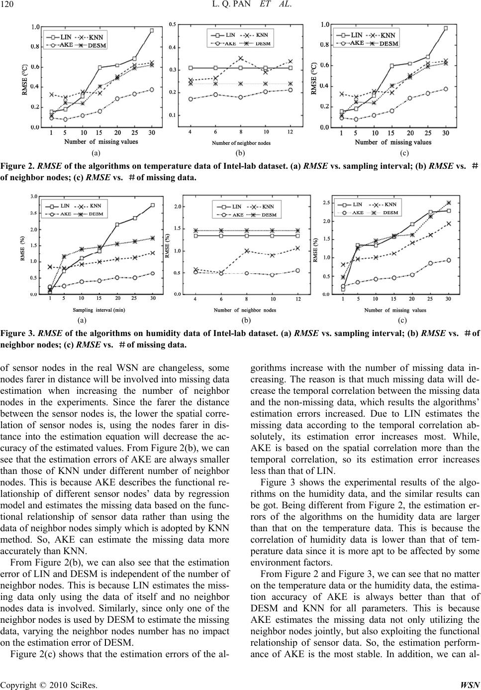 L. Q. PAN ET AL. Copyright © 2010 SciRes. WSN 120 (a) (b) (c) Figure 2. RMSE of the algorithms on temperature data of Intel-lab dataset. (a) RMSE vs. sampling interval; (b) RMSE vs. # of neighbor nodes; (c) RMSE vs. #of missing data. (a) (b) (c) Figure 3. RMSE of the algorithms on humidity data of Intel-lab dataset. (a) RMSE vs. sampling interval; (b) RMSE vs. #of neighbor nodes; (c) RMSE vs. #of missing data. gorithms increase with the number of missing data in- creasing. The reason is that much missing data will de- crease the temporal correlation between the missing data and the non-missing data, which results the algorithms’ estimation errors increased. Due to LIN estimates the missing data according to the temporal correlation ab- solutely, its estimation error increases most. While, AKE is based on the spatial correlation more than the temporal correlation, so its estimation error increases less than that of LIN. of sensor nodes in the real WSN are changeless, some nodes farer in distance will be involved into missing data estimation when increasing the number of neighbor nodes in the experiments. Since the farer the distance between the sensor nodes is, the lower the spatial corre- lation of sensor nodes is, using the nodes farer in dis- tance into the estimation equation will decrease the ac- curacy of the estimated values. From Figure 2(b), we can see that the estimation errors of AKE are always smaller than those of KNN under different number of neighbor nodes. This is because AKE describes the functional re- lationship of different sensor nodes’ data by regression model and estimates the missing data based on the func- tional relationship of sensor data rather than using the data of neighbor nodes simply which is adopted by KNN method. So, AKE can estimate the missing data more accurately than KNN. Figure 3 shows the experimental results of the algo- rithms on the humidity data, and the similar results can be got. Being different from Figure 2, the estimation er- rors of the algorithms on the humidity data are larger than that on the temperature data. This is because the correlation of humidity data is lower than that of tem- perature data since it is more apt to be affected by some environment factors. From Figure 2(b), we can also see that the estimation error of LIN and DESM is independent of the number of neighbor nodes. This is because LIN estimates the miss- ing data only using the data of itself and no neighbor nodes data is involved. Similarly, since only one of the neighbor nodes is used by DESM to estimate the missing data, varying the neighbor nodes number has no impact on the estimation error of DESM. From Figure 2 and Figure 3, we can see that no matter on the temperature data or the humidity data, the estima- tion accuracy of AKE is always better than that of DESM and KNN for all parameters. This is because AKE estimates the missing data not only utilizing the neighbor nodes jointly, but also exploiting the functional relationship of sensor data. So, the estimation perform- ance of AKE is the most stable. In addition, we can al- Figure 2(c) shows that the estimation errors of the al-  L. Q. PAN ET AL.121 sosee that, with the increasing of the sampling time in- terval and the number of missing data, the estimation effect of AKE is much better than that of the other algo- rithms. This is also because the same reasons. 4.2. Redwood Dataset Figure 4 and Figure 5 show the experimental results of the algorithms on temperature and humidity data of the Red- wood dataset respectively. From these two figures, we can see the similar experimental results with those of the In- tel-lab dataset. The difference is that, on the Redwood dataset, the performance of LIN decreases more greatly when the sampling time interval or the number of missing data increases. This is because the data of the Redwood dataset is collected by the WSN deployed outdoors. The data of outdoors changes more sharply and irregularly, which makes the temporal correlation of the sensor data be lower. Thus, the estimation performance of LIN is worse on the Redwood dataset. Comparatively, due to AKE is based on the spatial correlation more than the temporal correlation, its performance remains relative stable. From Figure 4 and Figure 5, we note that even KNN which is a naive spatial correlation based missing data estimation algorithm always outperforms LIN for all parameters, especially on humidity data. Thus, we can conclude that, for the data of changing non-smoothly, the spatial correlation based missing data estimation algo- rithms will perform better. From Figure 4 and Figure 5, we can also see that the performance gap between AKE and KNN is not too much on the Redwood dataset, especially on humidity data. This is mainly because the sensor data of outdoors changes more sharply and irregularly, the sensor data is in a low correlation. This decreases the advantage of the regression equation, and hence shrinks the performance gap between AKE and KNN. However, no matter in what cases, we can see that AKE always performs the best. 5. Conclusions Missing data causes many difficulties in various applica- tions of WSNs. Whereas, it is inevitable due to the in- herent characteristic of WSNs. To solve the problem, the best way is to estimate the missing data as accurately as possible. In this paper, a k-nearest neighbor based miss- ing data estimation algorithm, called AKE, is proposed. The algorithm is based on the spatial correlation more than the temporal correlation of sensor data, and esti- mates the missing data utilizing multiple neighbor nodes (a) (b) (c) Figure 4. RMSE of the algorithms on temperature data of redwood dataset. (a) RMSE vs. sampling interval; (b) RMSE vs. # of neighbor nodes; (c) RMSE vs. #of missing data. (a) (b) (c) Figure 5. RMSE of the algorithms on humidity data of redwood dataset. (a) RMSE vs. sampling interval; (b) RMSE vs. #of neighbor nodes; (c) RMSE vs. #of missing data. Copyright © 2010 SciRes. WSN  L. Q. PAN ET AL. 122 jointly rather than independently. So, the estimation per- formance of the algorithm is stable and reliable. In addi- tion, the algorithm estimates the missing data by ex- ploiting the functional relationship of sensor data rather than using the sensor data directly, so, the estimated val- ues computed by AKE are more accurate. Experimental results on two real-world datasets show that the algo- rithm proposed in this paper performs well both for the data indoors and the data outdoors. 6. Acknowledgments This work is partially supported by the Key Program of the National Natural Science Foundation of China under Grant No.60533110, the National Grand Fundamental Research 973 Program of China under Grant No.2006 CB303005, the National Natural Science Foundation of China under Grant No.60773063 and No.60703012, and the NSFC-RGC of China under Grant No. 60831160525. 7 . References [1] D. E. Cullar, D. Estrin, and M. Strvastava, “Overview of sensor networks,” IEEE Computer, Vol. 37, No. 8, pp. 41–49, 2004. [2] W. F. Fung, D. Sun, and J. Gehrke, “Cougar: the network is the database,” In SIGMOD Conference, pp. 621, 2002. [3] S. Madden, M. J. Franklin, J. M. Hellerstein, and W. Hong, “The design of an acquisitional query processor for sensor networks [C],” In SIGMOD. San Diego, Califor- nia, 2003. [4] Y. Yao and J. Gehrke, “The cougar approach to in- network query processing in sensor networks,” In SIGMOD Record, Vol. 31, No. 3, pp. 9–18, 2002. [5] G. Tolle, “Sonoma redwoods data,” 2005. http://www.cs. berkeley.edu/~get/sonoma/. [6] S. Madden, “Intel Berkeley research lab data,” 2003. http://berkeley.intel-research.net/labdata. [7] X. Zhu, S. Zhang, J. Zhang, and C. Zhang, “Cost- sensitive imputing missing values with ordering,” In AAAI. Vancouver, Canada, pp. 1922–1923, 2007. [8] N. A. Setiawan, P. A. Venkatachalam, and A. F. M. Hani, “Missing attribute values prediction based on artificial neural network and rough set theory,” In BMEI. Sanya, Hainan, China, pp. 306–310, 2008. [9] M. S. B. Sehgal, I. Gondal, L. Dooley, and R. L. Coppel, “Ameliorative missing value imputation for robust biological knowledge inference,” Journal of Biomedical Informatics, Vol. 41, No. 4, pp. 499–514, 2008. [10] M. S. B. Sehgal, I. Gondal, and L. Dooley, “Collateral missing value imputation: A new robust missing value estimation algorithm for microarray data,” Bioinformatics, Vol. 21, No. 10, pp. 2417–2423, 2005. [11] H. Kim, G. H. Golub, and H. Park., “Missing value estimation for dna microarray gene expression data: local least squares imputation[J],” Bioinformatics, Vol. 22, No. 11, pp. 1410–1411, 2006. [12] O. G. Troyanskaya, M. Cantor, G. Sherlock, P. O. Brown, T. Hastie, R. Tibshirani, D. Botstein, and R. B. Altman, “Missing value estimationmethods for dna microarrays,” Bioinformatics, Vol. 17, No. 6, pp. 520–525, 2001. [13] C. Zhang, X. Zhu, J. Zhang, Y. Qin, and S. Zhang, “Gbkii: An imputation method for missing values,” In PAKDD. Nanjing, China, pp. 1080–1087, 2007. [14] S. Zhang, J. Zhang, X. Zhu, Y. Qin, and C. Zhang, “Missing value imputation based on data clustering,” Transactions on Computational Science, Vol. 1, No. 1, pp. 128–138, 2008. [15] A. Manjhi, S. Nath, and P. B. Gibbons, “Tributaries and deltas: efficient and robust aggregation in sensor network streams,” In SIGMOD Conference. Baltimore, Maryland, pp. 287–298, 2005. [16] A. Silberstein, K. Munagala, and J. Yang, “Energy- efficient monitoring of extreme values in sensor networks,” In SIGMOD Conference. Chicago, Illinois, pp. 169–180, 2006. [17] D. J. Abadi, S. Madden, and W. Lindner, “Reed: robust, efficient filtering and event detection in sensor networks,” In VLDB, Trondheim, Norway, pp. 769–780, 2005. [18] X. Yang, H. B. Lim, M. T. Ozsu, and K. L. Tan. “In- network execution of monitoring queries in sensor networks,” In SIGMOD Conference, Beijing, China, pp. 521–532, 2007. [19] J. Considine, F. Li, G. Kollios, and J. Byers, “Approximate aggregation techniques for sensor data- bases,” In ICDE. Boston, MA, pp. 449–460, 2004. [20] A. Deshpande, C. Guestrin, S. Madden, J. M. Hellerstein, and W. Hong, “Model-driven data acquisition in sensor networks,” In VLDB, Toronto, Canada, pp. 588–599, 2004. [21] A. Deshpande, C. Guestrin, W. Hong, and S. Madden, “Exploiting correlated attributes in axquisitional query processing,” In ICDE, Tokyo, Japan, pp. 143–154, 2005. [22] D. Chu, A. Deshpand, J. M. Hellerstein, and W. Hong, “Approximate data collection in sensor networks using probabilistic models,” In ICDE. Atlanta, pp. 48, 2006. [23] A. Silberstein, R. Braynard, C. S. Ellis, K. Munagala, and J. Yang, “A sampling-based approach to optimizing top-k queries in sensor networks,” In ICDE. Atlanta, pp. 68, 2006. [24] Y. Li, C. Ai, W. P. Deshmukh, and Y. Wu, “Data estimation in sensor networks using physical and statistical methodologies,” In ICDCS, Beijing, China, pp. 538–545, 2008. [25] H. Zhang, J. M. F. Moura, and B. H. Krogh. “Estimation in sensor networks: A graph approach,” In IPSN, Los Angeles, California, pp. 203–209, 2005. [26] M. Halatchev and L. Gruenwald. “Estimating missing values in related sensor data streams,” In COMAD, Hyderabad, India, pp. 83–94, 2005. [27] N. Jiang and L. Gruenwald, “Estimating missing data in data streams,” In DASFAA, Bangkok, Thailand, pp. 981–987, 2007. C opyright © 2010 SciRes. WSN |