Wireless Sensor Network, 2010, 2, 108-114
doi:10.4236/wsn.2010.22015 Published Online February 2010 (http://www.SciRP.org/journal/wsn/).
Linear Pulse-Coupled Oscillators Model—A New
Approach for Time Synchronization in
Wireless Sensor Networks
Zhulin An1,2, Hongsong Zhu1,3, Meilin Zhang1, Chaonong Xu4, Yongjun Xu1, Xiaowei Li1
1Institute of Computing Technology, Chinese Academy of Sciences, Beijing, China
2Graduate University of Chinese Academy of Sciences, Beijing, China
3Institute of Software, Chinese Academy of Sciences, Beijing, China
4Department of Computer Science and Technology, China University of Petroleum-Beijing, Beijing, China
Received November 13, 2009; revised December 14, 2009; accepted December 7, 2009
Abstract
Mutual synchronization is a ubiquitous phenomenon that exists in various natural systems. The individual
participants in this process can be modeled as oscillators, which interact by discrete pulses. In this paper, we
analyze the synchronization condition of two- and multi-oscillators system, and propose a linear pulse-cou-
pled oscillators model. We prove that the proposed model can achieve synchronization for almost all condi-
tions. Numerical simulations are also included to investigate how different model parameters affect the syn-
chronization. We also discuss the implementation of the model as a new approach for time synchronization
in wireless sensor networks.
Keywords: Synchronization, Biologically Inspired Algorithms, Pulse-Coupled Oscillators, Wireless Sensor
Networks
1. Introduction
Synchronous flashing of fireflies is a fascinating phe-
nomenon that a large number of scientists have been
drawn to research on. The mechanism behind this phe-
nomenon has been investigated for nearly a century. In
1915, Blair observed and tried to examine the scientific
reason behind it [1]. He analogize firefly to electric bat-
tery—each flash temporarily exhausts the battery, and a
period of recuperation is required before the next flash
can be emitted. The flash of a leader stimulates the dis-
charge of others, and in the end this makes all the fireflies
flash in concert. Richmond presented a similar postula-
tion that if one firefly is ready to flash and sees flashes of
others, it starts sooner than otherwise [2]. In 1988, Buck
summarized these two battery-analogy mechanisms, and
proposed the phase-advanced model. He defined “late
sensitivity window” which is a time interval during the
period between a firefly’s flashings, and concluded that
when a photic stimulus (flashing) occurs during the late
sensitivity window, it initiates an immediate flash and
resets the status of the firefly.
Although the phase-advanced model gives a fine ex-
planation to certain varieties of fireflies’ synchronization
behavior, the interaction, which is usually called cou-
pling, between fireflies is narrowly limited to late sensi-
tivity window. Peskin extended coupling to any time of
the cycle. In his book published in 1975 [3], Peskin pro-
posed a more detailed pulse-coupled oscillators model
for the natural pacemaker of a human heart. He modeled
a pacemaker as a system consisting of mutual coupled
“integrate-and-fire” oscillators. Each oscillator is char-
acterized by state
x
, which satisfies
0
dx
x
S
dt


 01
x
 (1)
where

and 0 S are intrinsic properties of the oscil-
lators. When 1x

an oscillator fires then jumps back
to 0x

, and the states of the other oscillators will be
kicked up by coupling strength

. Through his research,
Peskin found that due to coupling, the states of the oscil-
lators tend to come to the same. And as the system
evolves, all oscillators would eventually achieve the state
of discharging in steps. Peskin proved that for a two os-
cillators system with small

and

, the system ap-
proaches a state in which the oscillators are firing syn-
chronously. Mirollo and Strogatz extended Peskin’s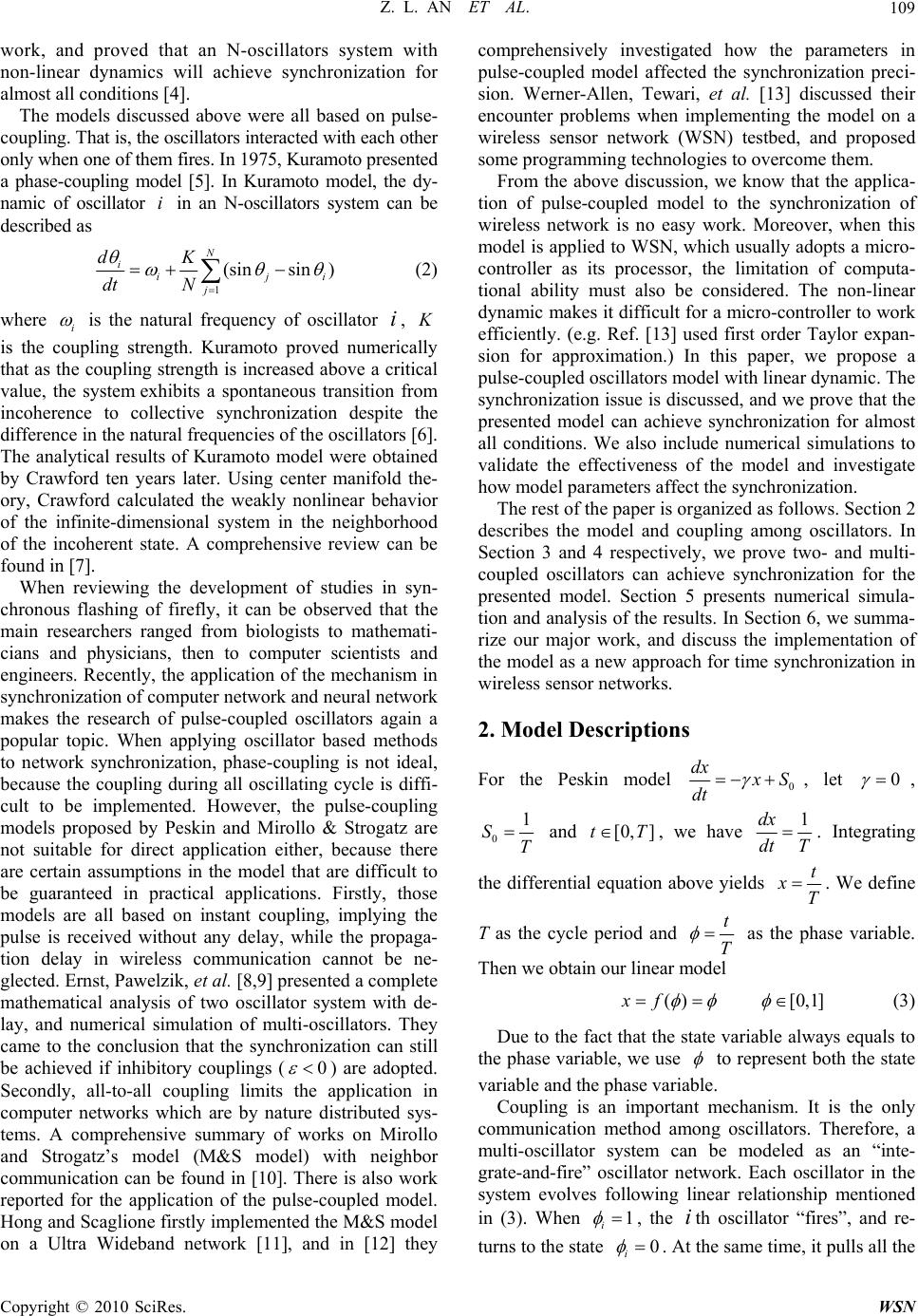

Z. L. AN ET AL. 109
work, and proved that an N-oscillators system with
non-linear dynamics will achieve synchronization for
almost all conditions [4].
The models discussed above were all based on pulse-
coupling. That is, the oscillators interacted with each other
only when one of them fires. In 1975, Kuramoto presented
a phase-coupling model [5]. In Kuramoto model, the dy-
namic of oscillator i in an N-oscillators system can be
described as
1
(sinsin )
N
i
iji
j
dK
dt N




 
 (2)
where i

is the natural frequency of oscillator i,
K
is the coupling strength. Kuramoto proved numerically
that as the coupling strength is increased above a critical
value, the system exhibits a spontaneous transition from
incoherence to collective synchronization despite the
difference in the natural frequencies of the oscillators [6].
The analytical results of Kuramoto model were obtained
by Crawford ten years later. Using center manifold the-
ory, Crawford calculated the weakly nonlinear behavior
of the infinite-dimensional system in the neighborhood
of the incoherent state. A comprehensive review can be
found in [7].
When reviewing the development of studies in syn-
chronous flashing of firefly, it can be observed that the
main researchers ranged from biologists to mathemati-
cians and physicians, then to computer scientists and
engineers. Recently, the application of the mechanism in
synchronization of computer network and neural network
makes the research of pulse-coupled oscillators again a
popular topic. When applying oscillator based methods
to network synchronization, phase-coupling is not ideal,
because the coupling during all oscillating cycle is diffi-
cult to be implemented. However, the pulse-coupling
models proposed by Peskin and Mirollo & Strogatz are
not suitable for direct application either, because there
are certain assumptions in the model that are difficult to
be guaranteed in practical applications. Firstly, those
models are all based on instant coupling, implying the
pulse is received without any delay, while the propaga-
tion delay in wireless communication cannot be ne-
glected. Ernst, Pawelzik, et al. [8,9] presented a complete
mathematical analysis of two oscillator system with de-
lay, and numerical simulation of multi-oscillators. They
came to the conclusion that the synchronization can still
be achieved if inhibitory couplings (0

) are adopted.
Secondly, all-to-all coupling limits the application in
computer networks which are by nature distributed sys-
tems. A comprehensive summary of works on Mirollo
and Strogatz’s model (M&S model) with neighbor
communication can be found in [10]. There is also work
reported for the application of the pulse-coupled model.
Hong and Scaglione firstly implemented the M&S model
on a Ultra Wideband network [11], and in [12] they
comprehensively investigated how the parameters in
pulse-coupled model affected the synchronization preci-
sion. Werner-Allen, Tewari, et al. [13] discussed their
encounter problems when implementing the model on a
wireless sensor network (WSN) testbed, and proposed
some programming technologies to overcome them.
From the above discussion, we know that the applica-
tion of pulse-coupled model to the synchronization of
wireless network is no easy work. Moreover, when this
model is applied to WSN, which usually adopts a micro-
controller as its processor, the limitation of computa-
tional ability must also be considered. The non-linear
dynamic makes it difficult for a micro-controller to work
efficiently. (e.g. Ref. [13] used first order Taylor expan-
sion for approximation.) In this paper, we propose a
pulse-coupled oscillators model with linear dynamic. The
synchronization issue is discussed, and we prove that the
presented model can achieve synchronization for almost
all conditions. We also include numerical simulations to
validate the effectiveness of the model and investigate
how model parameters affect the synchronization.
The rest of the paper is organized as follows. Section 2
describes the model and coupling among oscillators. In
Section 3 and 4 respectively, we prove two- and multi-
coupled oscillators can achieve synchronization for the
presented model. Section 5 presents numerical simula-
tion and analysis of the results. In Section 6, we summa-
rize our major work, and discuss the implementation of
the model as a new approach for time synchronization in
wireless sensor networks.
2. Model Descriptions
For the Peskin model 0
dx
x
S
dt
  , let 0


,
0
1
ST

and [0, ]tT

, we have 1dx
dt T
. Integrating
the differential equation above yields t
xT . We define
T as the cycle period and t
T
  as the phase variable.
Then we obtain our linear model
()xf



 [0,1]

 (3)
Due to the fact that the state variable always equals to
the phase variable, we use

to represent both the state
variable and the phase variable.
Coupling is an important mechanism. It is the only
communication method among oscillators. Therefore, a
multi-oscillator system can be modeled as an “inte-
grate-and-fire” oscillator network. Each oscillator in the
system evolves following linear relationship mentioned
in (3). When 1
i


, the ith oscillator “fires”, and re-
turns to the state 0
i


. At the same time, it pulls all the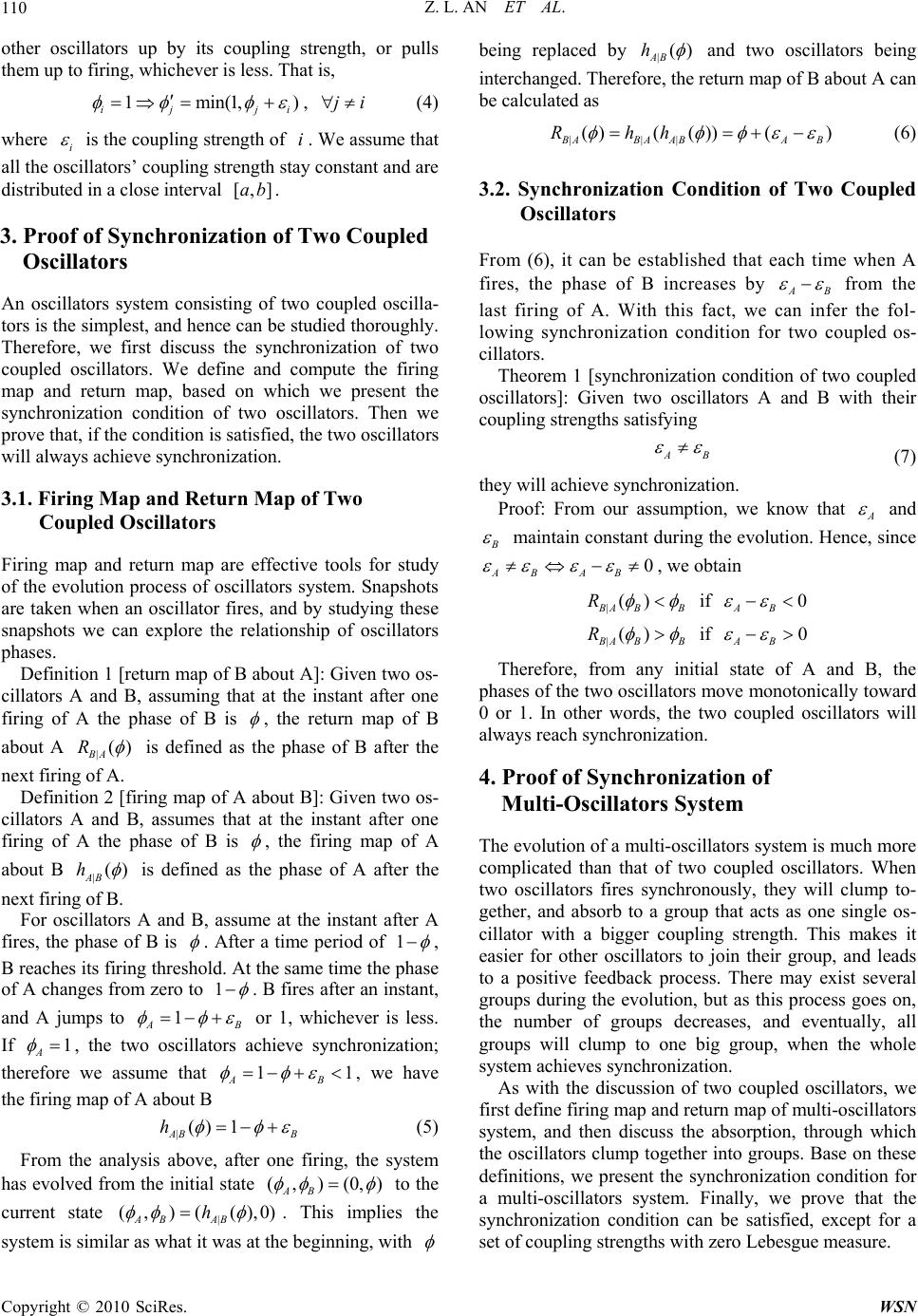

Z. L. AN ET AL. 110
other oscillators up by its coupling strength, or pulls
them up to firing, whichever is less. That is,
1min(1,)
ij ji
 


 , ji (4)
where i

is the coupling strength of i. We assume that
all the oscillators’ coupling strength stay constant and are
distributed in a close interval [,]ab .
3. Proof of Synchronization of Two Coupled
Oscillators
An oscillators system consisting of two coupled oscilla-
tors is the simplest, and hence can be studied thoroughly.
Therefore, we first discuss the synchronization of two
coupled oscillators. We define and compute the firing
map and return map, based on which we present the
synchronization condition of two oscillators. Then we
prove that, if the condition is satisfied, the two oscillators
will always achieve synchronization.
3.1. Firing Map and Return Map of Two
Coupled Oscillators
Firing map and return map are effective tools for study
of the evolution process of oscillators system. Snapshots
are taken when an oscillator fires, and by studying these
snapshots we can explore the relationship of oscillators
phases.
Definition 1 [return map of B about A]: Given two os-
cillators A and B, assuming that at the instant after one
firing of A the phase of B is

, the return map of B
about A |()
BA
R

is defined as the phase of B after the
next firing of A.
Definition 2 [firing map of A about B]: Given two os-
cillators A and B, assumes that at the instant after one
firing of A the phase of B is

, the firing map of A
about B |()
AB
h

is defined as the phase of A after the
next firing of B.
For oscillators A and B, assume at the instant after A
fires, the phase of B is

. After a time period of 1


,
B reaches its firing threshold. At the same time the phase
of A changes from zero to 1


. B fires after an instant,
and A jumps to 1
AB

  or 1, whichever is less.
If 1
A

, the two oscillators achieve synchronization;
therefore we assume that 11
AB



 , we have
the firing map of A about B
|() 1 AB B
h

   (5)
From the analysis above, after one firing, the system
has evolved from the initial state (,)(0,)
AB
 
 to the
current state | (,)( (),0)
AB AB
h
 
. This implies the
system is similar as what it was at the beginning, with

being replaced by |()
AB
h

and two oscillators being
interchanged. Therefore, the return map of B about A can
be calculated as
|||
()( ())()
B
ABAAB AB
Rhh



  (6)
3.2. Synchronization Condition of Two Coupled
Oscillators
From (6), it can be established that each time when A
fires, the phase of B increases by AB

  from the
last firing of A. With this fact, we can infer the fol-
lowing synchronization condition for two coupled os-
cillators.
Theorem 1 [synchronization condition of two coupled
oscillators]: Given two oscillators A and B with their
coupling strengths satisfying
AB



(7)
they will achieve synchronization.
Proof: From our assumption, we know that A

and
B

maintain constant during the evolution. Hence, since
0
AB AB



, we obtain
|()
B
AB B
R


if 0
AB

 
|()
B
AB B
R

 if 0
AB

 
Therefore, from any initial state of A and B, the
phases of the two oscillators move monotonically toward
0 or 1. In other words, the two coupled oscillators will
always reach synchronization.
4. Proof of Synchronization of
Multi-Oscillators System
The evolution of a multi-oscillators system is much more
complicated than that of two coupled oscillators. When
two oscillators fires synchronously, they will clump to-
gether, and absorb to a group that acts as one single os-
cillator with a bigger coupling strength. This makes it
easier for other oscillators to join their group, and leads
to a positive feedback process. There may exist several
groups during the evolution, but as this process goes on,
the number of groups decreases, and eventually, all
groups will clump to one big group, when the whole
system achieves synchronization.
As with the discussion of two coupled oscillators, we
first define firing map and return map of multi-oscillators
system, and then discuss the absorption, through which
the oscillators clump together into groups. Base on these
definitions, we present the synchronization condition for
a multi-oscillators system. Finally, we prove that the
synchronization condition can be satisfied, except for a
set of coupling strengths with zero Lebesgue measure.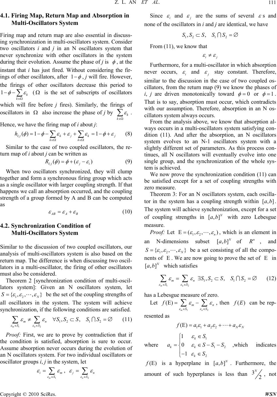

Z. L. AN ET AL. 111
4.1. Firing Map, Return Map and Absorption in
Multi-Oscillators System
Firing map and return map are also essential in discuss-
ing synchronization in multi-oscillators system. Consider
two oscillators i and j in an N oscillators system that
never synchronize with other oscillators in the system
during their evolution. Assume the phase of j is

, at the
instant that i has just fired. Without considering the fir-
ings of other oscillators, after 1

, j will fire. However,
the firings of other oscillators decrease this period to
1k
k




 ( is the set of subscripts of oscillators
which will fire before j fires). Similarly, the firings of
oscillators in  also increase the phase of j by k
k



.
Hence, we have the firing map of i about j:
|() 11 ijk jkj
kk
h

 
 
  
 (8)
Similar to the case of two coupled oscillators, the re-
turn map of i about j can be written as
|() () ijj i
R

  (9)
When two oscillators synchronized, they will clump
together and form a synchronous firing group which acts
as a single oscillator with larger coupling strength. If that
happens we call an absorption occurred, and the coupling
strength of a group formed by A and B can be computed
as
ABAB

  (10)
4.2. Synchronization Condition of
Multi-Oscillators System
Similar to the discussion of two coupled oscillators, our
analysis of multi-oscillators system is also based on the
return map. The difference is when discussing two oscil-
lators in a multi-oscillator, the firing of other oscillators
must also be considered.
Theorem 2 [synchronization condition of multi-oscil-
lators system]: Given an N oscillators system, let
12
{, ,,}
N
S

  be the set of the coupling strengths of
all oscillators in the system. The system will achieve
synchronization, if the following conditions are satisfied.
12mn
mn
SS 





121 2 ,,SSS SS  (11)
Proof: First, we are to prove by contradiction that if
the condition is satisfied, absorption is sure to occur.
Assume absorption never occurs during the evolution of
an N oscillators system. For two individual oscillators or
oscillator groups i, j in the system, let
1m
im
S 



,
2n
j
n
S 




Since i

and
j

are the sums of several

s and
none of the oscillators in i and j are identical, we have
1212
,,SSS S S
From (11), we know that
ij



Furthermore, for a multi-oscillator in which absorption
never occurs, i

and j

stay constant. Therefore,
similar to the discussion in the case of two coupled os-
cillators, from the return map (9) we know the phases of
i, j are driven monotonically toward 0

 or 1


.
That is to say, absorption must occur, which contradicts
with our assumption. Therefore, absorption in an N os-
cillators system always occurs.
From the analysis above, we know that absorption al-
ways occurs in a multi-oscillators system satisfying con-
dition (11). And after the absorption, an N oscillators
system evolves to an N-1 oscillators system with a
slightly different set of parameters. As this process con-
tinues, all N oscillators will eventually evolve into one
single group, and the synchronization of the whole sys-
tem is achieved.
We now prove the synchronization condition (11) can
be satisfied except for a set of coupling strengths with
zero measure.
Theorem 3: For an N oscillators system, each oscilla-
tor in the system has a coupling strength within [,]ab .
The system will achieve synchronization, except for a set
of coupling strengths in [,]
N
ab with zero Lebesgue
measure.
Proof: Let 12
(, ,,)
n



, which is an element in
an N-dimensions subset [,]N ab of n R, and
12
{, ,,}
N
S



 be a set consisting of all the compo-
nents of

. We are now going to prove the set of

in
[, ]
N
ab which satisfies
12mn
mn
SS 





121 2
,,SSS S S

 (12)
has a Lebesgue measure of zero.
Let
12
()
mn
mn
SS
f




 

, then ()
f
E can be rep-
resented as
112 2
() NN faaa



 
where
1
12
2
1
0
1
k
kk
k
S
aSSS
S











,which indicates
()f

is a hyperplane in [,]
N
ab . Furthermore, the
amount of such hyperplanes is less than 32
N, not

Z. L. AN ET AL. 112
unlimited. Therefore, the set of  satisfying condition
(12) has the a Lebesgue measure of zero.
With Theorem 2, we found the synchronization condi-
tion for a multi-oscillators system, and proved if the con-
dition is satisfied the system will achieve synchroniza-
tion. Then in Theorem 3, we proved the condition will be
satisfied except for a set of coupling strengths with zero
measure. Combining the two theorems, we proved the
presented multi-oscillators system will achieve synchro-
nization except for a set of coupling strengths with zero
measures.
5. Numerical Simulation and Analysis
To validate that the synchronization can be established
for the presented model and investigate how model pa-
rameters affect the synchronization process, we perform
a numerical simulation of the model in a Java environ-
ment. Every simulation consists of an initialization stage
and a simulation stage. In the former, the parameters of
the model are initialized, which includes the number of
oscillators (n), the period (T), oscillator phase (

) and
coupling strength (

). Due to the limitation of computer
(a)
(b)
Figure 1. Phase and standard deviation of phase during the
synchronization process with n = 100, _base = 0.005,
_ratio = 0.1.
0.0 0.2 0.4 0.6 0.8 1.0
0
20
40
60
80
100
120
140
160
Cycles to Sync
ε Interval Ratio
n=10
n=100
n=1000
Figure 2. Cycle numbers to achieve synchronization versus
_ratio with _base = 0.01 for n = 10, 100 and 1000.
0200400600800 1000
0
5
10
15
20
25
Cycles to Sync
n
ε base value = 0.005
ε base value = 0.01
ε base value = 0.02
Figure 3. Cycle numbers to achieve synchronization versus
n with _ratio = 0.1 for various _base. Because when n and
_base are both very small, the cycle numbers until syn-
chronization is going to be very large. To show the detail of
all the plots, the figure is ploted from n = 50.
simulation, T,

and

are all discretized to inte-
gers. Specifically, T is set to a large number
(10000000), and

is generated randomly between [0,
T].

is generated randomly between [_base

1
_
*_ ,
2base ratio
 1
_
_
2
base

 *base

_ratio ],
where _base

, _ratio

are “coupling strength base
value” and “coupling strength interval ratio” respectively.
The simulation stage consists of many cycles. During
each cycle, the oscillator with the maximum phase is
found first, and the system is forwarded to the firing in-
stant of the oscillator. Then all the oscillators’ phases are
adjusted according to the coupling strength of the fired
oscillator. Finally, all the fired oscillators are combined
into a group with new coupling strength computed by
(10). This cycle repeats until there is only one group left.

Z. L. AN ET AL. 113
Additionally, to avoid the effect of arbitrary randomness
of

and

, every simulation related to cycles to syn-
chronization is done 1000 times, and the average of 800
values in the center range (eliminate the maximum 100
results and the minimum 100 results) is adopted as the
final result.
We first simulate the synchronization process. The re-
sults are shown in Figure 1. Figure 1(a) shows the phases
of oscillators at different cycles. Each dash in the figure
represents the phase of a particular oscillator or oscillator
group, and the phases are plotted every time when the
phase of oscillator No.0 returns to 0. (As a result, there is
always a dash at 0

) We can see from the plot that as
cycles continue, the number of dashes decrease, indicat-
ing that the oscillators gradually clump into groups. In
the end, when there is only one group left, the oscillators
achieve synchronization. Figure 1(b) shows the standard
deviation of the oscillators’ phases during the same
process. From the figure, we can find that at the begin-
ning the standard deviation generally increases as the
evolution progresses, but each time when absorption
happens the standard deviation decreases. Near the end,
when there are only two groups, the standard deviation
decreases dramatically, and finally reaches zero.
We then investigate how the parameters (n,_base

and _ratio

) affect the number of cycles needed to
achieve synchronization. Figure 2 shows required cycle
number to achieve synchronization as a function of
_ratio

with _base

= 0.01 for n = 10, 100 and
1000. From Figure 2, we can see that when n is big
enough the cycle number to synchronize does not change
with _ratio

. We now discuss the reason behind this
phenomenon. Suppose i is an oscillator in a
multi-oscillators system, then every time when i fires, its
phase increases by 1,
n
k
kki


. In this simulation, al-
though _ratio

varies, the sum of all

lies on
_base

. Furthermore when n is big enough, the sum
1,
n
k
kki


 will approximate the sum of all

. There-
fore, the cycles needed stay the same. We also notice that
when n and _ratio

are both small, more cycles are
needed to synchronize. This is because, if _ratio

is
small the

of all oscillators will be almost the same.
Due to the linear dynamic, the deviation of all the oscil-
lators’ phases increases slowly, so more cycles are
needed.
Following above analysis, we know that the _ratio

will not affect the result if n is not a very small number.
So we fix the value of _ratio

to 0.1 and discuss how
number of cycles needed to synchronize varies with dif-
ferent values of n and _base

.
Figure 3 shows number of cycles required to achieve
0.00 0.05 0.10 0.150.20 0.25 0.30 0.35 0.40
0
5
10
15
20
25
30
Cycles to Sync
ε base value
n = 10
n = 100
n = 1000
Figure 4. Cycle numbers to achieve synchronization versus
_base with _ratio = 0.1 for various n. Because when n and
_base are both too small, the cycle number to synchro-
nized is too large. To show the detail of all the plots, the
figure is plotted from_base = 0.015.
synchronization versus n for various _base

. For a
fixed _base

, cycle numbers decrease with the in-
crease of n. The reason is that the more oscillators there
are in the system, the easier it is for the oscillators to
absorb to synchronous firing groups. And the

of a
group is the sum of

of all oscillators in that group, so
it is equivalent to increase the

of the oscillator.
Therefore, system tends to synchronize earlier.
Figure 4 shows cycle numbers to achieve synchroniza-
tion versus _base

with
_
0.1ratio

 for various
values of n. In the figure, we can find that for a certain
number of oscillators, the larger

is, the less cycles
are needed to achieve synchronization. This is because
the return map increases with the increase of

, and the
system tends to synchronize faster.
From the simulation result presented in this section,
we can draw the following conclusion. First, as we dis-
cussed in Subsection 4.1, with the evolution of a
muti-oscillator system, the oscillators in the system tend
to clump together into synchronous firing groups. When
there is only one group left, the system achieves syn-
chronization. Second, the number of cycles to achieve
synchronization depends on n and _base

; a larger
n or _base

may lead to faster synchronization, and
_ratio

will have no effect on the number of cycles to
synchronize, unless n is very small. To summarize, the
simulations match well with our theoretical analysis.
6. Conclusions and Future Work
In this paper, we proposed a model for linear pulse-cou-
pled oscillators system with different coupling strengths.
We discussed the synchronization condition for both

Z. L. AN ET AL. 114
two- and multi-oscillators system, and proved that the
proposed system can achieve synchronization for almost
all conditions. Simulations of the model in a Java envi-
ronment are also included, which validated the model
and investigated how different parameters affect the
synchronization.
As a swarm of fireflies, a WSN consists of a number
of wireless sensor nodes that interact with each other via
radio communications. Therefore, if the model presented
in this paper is applied as a new approach for time syn-
chronization in WSNs, the algorithm would be more
scalable and robust. In the implement, the phase de-
scribed in the model is represented by a counter, which
moves monotonically towards a threshold T, corre-
sponding to the period of the oscillator. When the
counter reaches T, it jump back to zero and triggers an
interrupt follow with a new cycle. In the interrupt han-
dler, a packet containing the node’s coupling strength

is sent out, which will be used by other nodes to add to
their own counter. In this manner, all the counters will be
synchronized after a few cycles as what has been dis-
cussed in the simulation. However, there is also factors
must be considered before this model can be adopted
practically, including the message delay, the message
collision, the network topology and so on. The imple-
ment of the model on a WSN testbed will be included in
our future work.
7. Acknowledgement
The research presented in this paper was supported in
part by National Natural Science Foundation of China
(NSFC) under grants No.(60772070, 60873244, 60633060,
60831160526), in part by High-Tech Research and De-
velopment Program of China (863) under grants
No.(2007AA12Z321, 2007AA01Z113), and in part by
National Basic Research Program of China (973) under
grant No.(2005CB321604, 2006CB303000). Authors
also wish to acknowledge help of Sen Yu in writing the
English version of this paper.
8. References
[1] K. G. Blair, “Luminous Insects,” Nature, Vol. 96, No.
2406, pp. 411–415, 1915.
[2] C. A. Richmond, “Fireflies flashing in unison,” Science,
Vol. 71, No. 1847, pp. 537–538, 1930.
[3] C. S. Peskin, “Self-synchronization of the cardiac pace-
maker,” in Mathematical Aspects of Heart Physiology,
New York University: New York. pp. 268–278, 1975.
[4] R. E. Mirollo and S. H. Strogatz, “Synchronization of
pulse-coupled biological oscillators,” SIAM Journal on
Applied Mathematics, Vol. 50, No. 6, pp. 1645–1662,
1990.
[5] Y. Kuramoto, “Self-entrainment of a population of cou-
pled non-linear oscillators,” in International Symposium
on Mathematical Problems in Theoretical Physics, pp.
420–422, 1975.
[6] Y. Kuramoto, “Chemical oscillations, waves, and turbu-
lence,” Springer Series in Synergetics, Berlin,
Springer-Verlag, pp. 164, 1984.
[7] S. H. Strogatz, “From kuramoto to crawford: exploring
the onset of synchronization in populations of coupled
oscillators,” Physica D: Nonlinear Phenomena, Vol. 143,
No.1–4, pp. 1–20, 2000.
[8] U. Ernst, K. Pawelzik, and T. Geisel, “Synchronization
induced by temporal delays in pulse-coupled oscillators,”
Physical Review Letters, Vol. 74, No. 9, pp. 1570–1573,
1995.
[9] U. Ernst, K. Pawelzik, and T. Geisel, “Delay-induced
multistable synchronization of biological oscillators,”
Physical Review E, Vol. 57, No. 2, pp. 2150–2162,
1998.
[10] O. Simeone, et al. “Distributed synchronization in wire-
less networks.” IEEE Signal Processing Magazine, Vol.
25, No. 5, pp. 81–97, 2008.
[11] Y. W. Hong and A. Scaglione, “Time synchronization
and reach-back communications with pulse-coupled os-
cillators for UWB wireless ad hoc networks,” in Pro-
ceedings of IEEE Conference on Ultra Wideband Sys-
tems and Technologies, 2003.
[12] Y. W. Hong, and A. Scaglione, “A scalable synchroniza-
tion protocol for large scale sensor networks and its ap-
plications,” IEEE Journal on Selected Areas in Commu-
nications, Vol. 23, No. 5, pp. 1085–1099, 2005.
[13] G. Werner-Allen, et al. “Firefly-inspired sensor network
synchronicity with realistic radio effects,” in Proceedings
of the 3rd international conference on Embedded net-
worked sensor systems. ACM: San Diego, California,
USA. pp. 142–153, 2005.
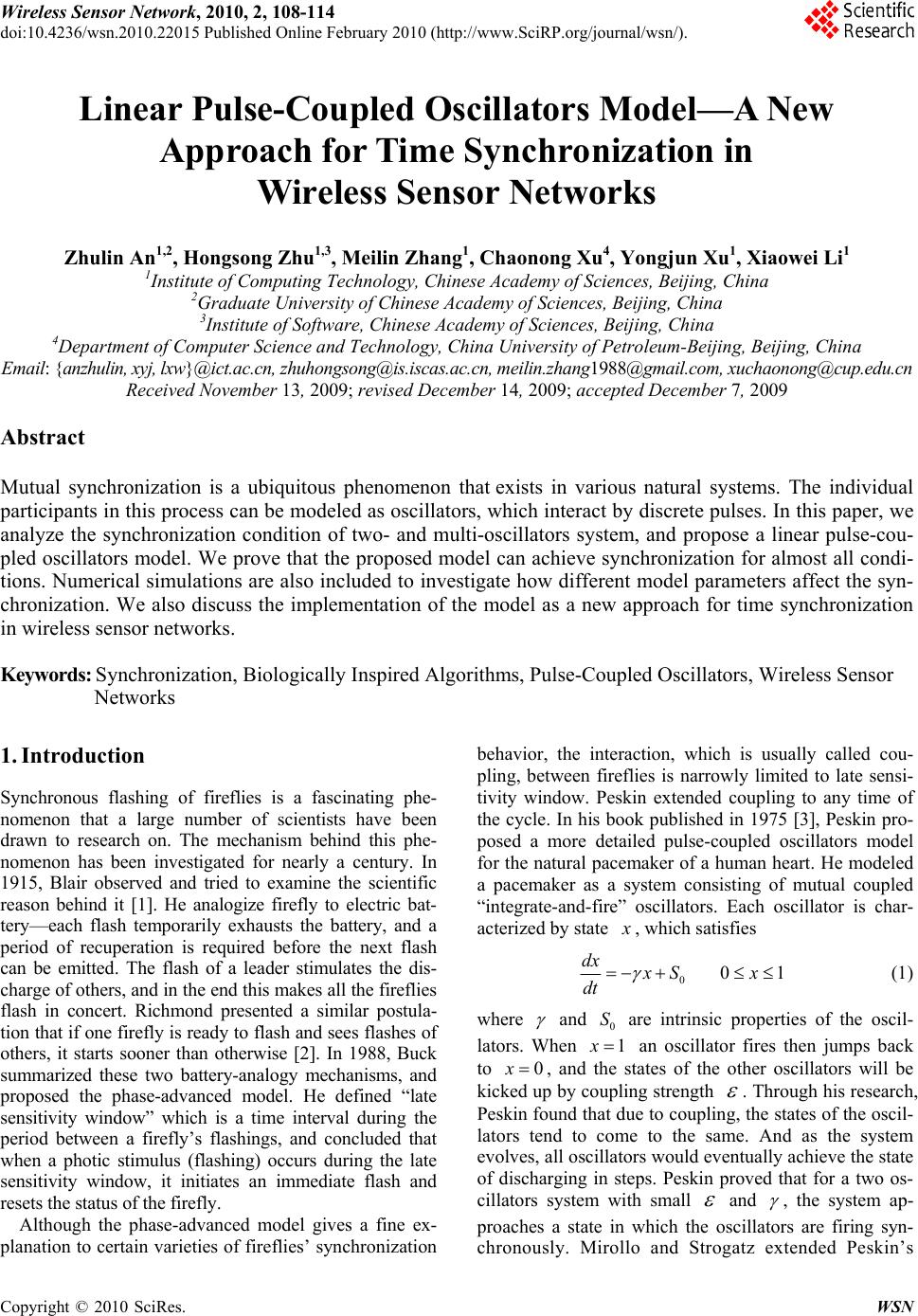