J. Software Engineering & Applications, 2010, 3: 185-189
doi:10.4236/jsea.2010.32023 Published Online February 2010 (http://www.SciRP.org/journal/jsea)
185
Research on LFS Algorithm in Software Network
Wei Wang, Hai Zhao, Hui Li, Jun Zhang, Peng Li, Zheng Liu, Naiming Guo, Jian Zhu, Bo Li,
Shuang Yu, Hong Liu, Kunzhan Yang
Information Science and E n g i n e e ri n g Northeastern University, Shenyang, China.
Received October 11th, 2009; revised October 26th, 2009; accepted November 5th, 2009.
ABSTRACT
Betweenness centrality helps researcher to master the changes of the system from the overall perspective in software
network. The existing betweenness centrality algorithm has high time complexity but low accuracy. Therefore, Layer
First Searching (LFS) algorithm is proposed that is low in time complexity and high in accuracy. LFS algorithm
searches the nodes with the shortest to the designated node, then travels all paths and calculates the nodes on the paths,
at last get the times of ea ch node being traveled which is betweenness centrality. Th e time complexity of LFS algorithm
is O(V2).
Keywords: LFS, Software Network, the Shortest Path, Betweenness Centrality
1. Introduction
It is over fifteen years since Norman Fenton outlined the
need for a scientific basis of software measurement. Such
a theory is a prerequisite for any useful quantitative ap-
proach to software engineering, although little attention
has been received from both practitioners and researchers.
Measurement is the process that assigns numbers or
symbols to attributes of real-world entities. Unfortunately,
many empirical studies of software measurements lack a
forecast system that combines measurements and pa-
rameters in order to make quantitative predictions. How
can we overcome these limitations?
Here we present a new approach to software engineer-
ing based on recent advances in complex networks. As a
typical parameter and an important global statistics, be-
tweenness centrality can meet the need s of researchers to
know the inter-reaction of software network from the
overall perspective. The definition of betweenness cen-
trality is the times of a node being traveled in all the
shortest paths of the software network and it reflects the
influence of the node in the whole network.
The existing betweenness centrality algorithms are ei-
ther based on the shortest path or merely approximate
algorithm [1–3], and both have its own shortcomings.
First, the traditional shortest path algorith m has high time
complexity and costs too much time to be available in
large network, which makes it impossible to put the al-
gorithms into practice. Th e research on approximation of
betweenness centrality is unavailable for low accuracy
which brings great obstacle for further study [4,5].
As mentioned in [6], the averag e path length is similar
to normal distribution with the mean of 15.21. LFS algo-
rithm is proposed based on this method.
The dissertation contains three parts: First, take
Dijkstra algorithm as example to conclude shortcomings
of traditional algorithms. Then, propose LFS algorithm.
At last, compare these two algorithms to show the ad-
vantages of LFS algorithm.
2. Traditional Dijkstra Algorithm
The complexity of betweenness centrality comes from
calculating the shortest path between each two nodes in
network, and the time complexity of Dijkstra is O(n3).
The existing algorithms based on the shortest path con-
tain Dijkstra, Floyd-Warshall, and Johnson. Dijkstra is
the most popular and classic algorithm.
The idea of Dijkstra is like this. Abstract the network
into a graph, Put the isolated nodes (the nodes with
out-degree and in-degree being both 0) in set V and the
nodes having been traveled in set S, then calculate the
shortest path from vi to any node in the graph. Move the
node vk with the shortest path from V-S to S till V-S is
empty.
① Initialization: Set up a two-dimensional array a to
mark whether the shortest path has been found out be-
tween the two nodes. Set up a none-dimensional array to
store the betweenness centrality. Set up a adjacency ma-
trix arcs with 1 if there exist edge between the nodes,
else with ∞. V is a set of all nodes and S is a set of all
marked nodes. The value from vi to vj is initializes as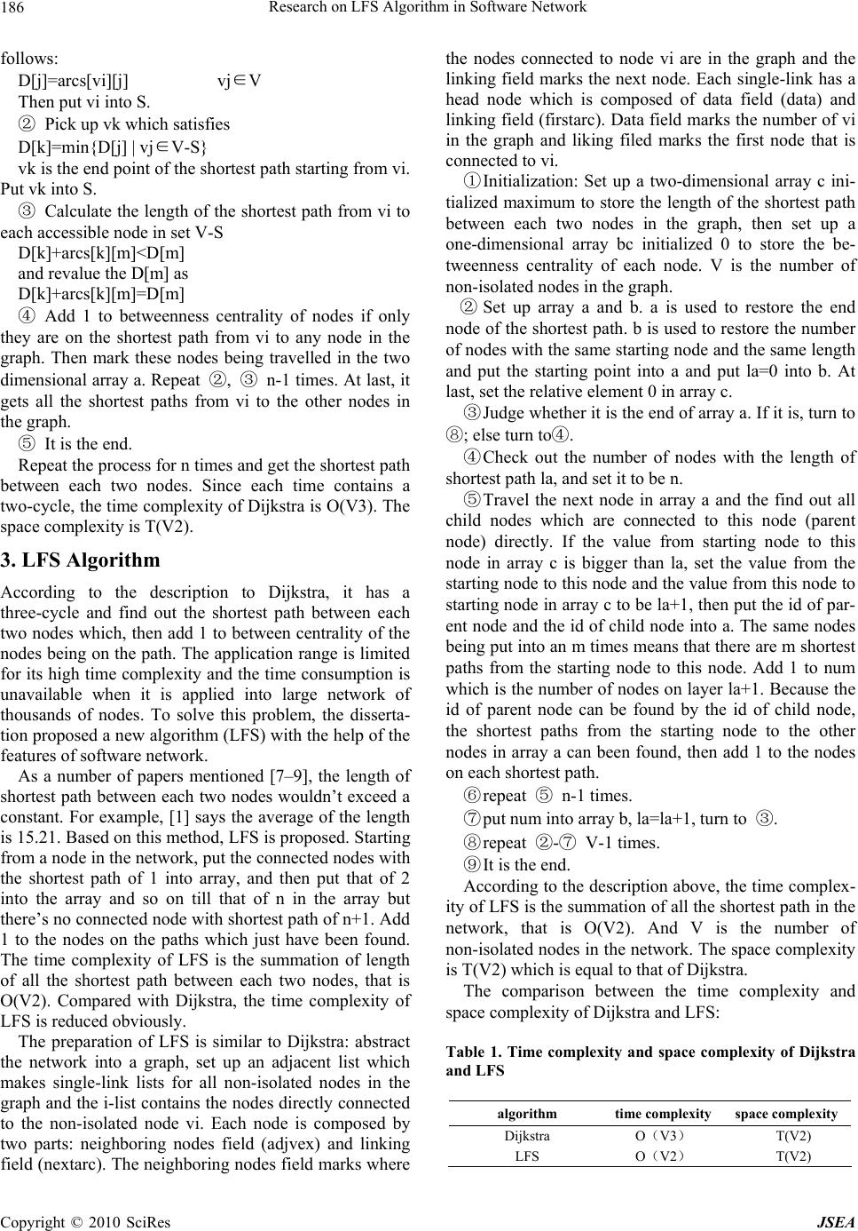

Research on LFS Algorithm in Software Network 186
follows:
D[j]=arcs[vi][j] vj∈V
Then put vi int o S.
② Pick up vk which satisfies
D[k]=min{D[j] | v j∈V-S}
vk is the end point of th e shortest p ath starting from vi.
Put vk into S.
③ Calculate the length of the shortest path from vi to
each accessible node in set V-S
D[k]+arcs[k][m]<D[m]
and revalue the D[m] as
D[k]+arcs[k][m]=D[m]
④ Add 1 to betweenness centrality of nodes if only
they are on the shortest path from vi to any node in the
graph. Then mark these nodes being travelled in the two
dimensional array a. Repeat ②, ③ n-1 times. At last, it
gets all the shortest paths from vi to the other nodes in
the graph.
⑤ It is the end.
Repeat the process for n times and get the shortest path
between each two nodes. Since each time contains a
two-cycle, the time complexity of Dijkstra is O(V3). The
space complexity is T(V2).
3. LFS Algorithm
According to the description to Dijkstra, it has a
three-cycle and find out the shortest path between each
two nodes which, then add 1 to between centrality of the
nodes being on the path . The application range is limited
for its high time complexity a nd the time consumption is
unavailable when it is applied into large network of
thousands of nodes. To solve this problem, the disserta-
tion proposed a new algorithm (LFS) w ith the help of the
features of software network.
As a number of papers mentioned [7–9], the length of
shortest path between each two nodes wouldn’t exceed a
constant. For example, [1] says the average of the length
is 15.21. Based on this method, LFS is proposed. Starting
from a node in the network, put the connected nodes with
the shortest path of 1 into array, and then put that of 2
into the array and so on till that of n in the array but
there’s no co nnected nod e with shortest p ath of n+1. Ad d
1 to the nodes on the paths which just have been found.
The time complexity of LFS is the summation of length
of all the shortest path between each two nodes, that is
O(V2). Compared with Dijkstra, the time complexity of
LFS is reduced obviously.
The preparation of LFS is similar to Dijkstra: abstract
the network into a graph, set up an adjacent list which
makes single-link lists for all non-isolated nodes in the
graph and the i-list contains the nodes directly connected
to the non-isolated node vi. Each node is composed by
two parts: neighboring nodes field (adjvex) and linking
field (nextar c). The neighboring nodes field marks wh ere
the nodes connected to node vi are in the graph and the
linking field marks the next node. Each single-link has a
head node which is composed of data field (data) and
linking field (firstarc). Data field marks the number of vi
in the graph and liking filed marks the first node that is
connected to vi.
① Initialization: Set up a two-dimensional array c ini-
tialized maximum to store the length of the shortest path
between each two nodes in the graph, then set up a
one-dimensional array bc initialized 0 to store the be-
tweenness centrality of each node. V is the number of
non-isolated nodes in the graph.
② Set up array a and b. a is used to restore the end
node of the shortest path. b is used to restore the number
of nodes with the same starting node and the same length
and put the starting point into a and put la=0 into b. At
last, set the relative element 0 in array c.
③ Judge whether it is the end of array a. If it is, turn to
⑧; else turn to④.
④ Check out the number of nodes with the length of
shortest path la, and set it to be n.
⑤ Travel the next node in array a and the find out all
child nodes which are connected to this node (parent
node) directly. If the value from starting node to this
node in array c is bigger than la, set the value from the
starting node to this node and the value from this node to
starting node in array c to be la+1, then pu t the id of par-
ent node and the id of child node into a. The same nodes
being put into an m times means that there are m shortest
paths from the starting node to this node. Add 1 to num
which is the number of nodes on layer la+1. Because the
id of parent node can be found by the id of child node,
the shortest paths from the starting node to the other
nodes in array a can been found, then add 1 to the nodes
on each shortest path.
⑥ repeat ⑤ n-1 times.
⑦ put num into array b, la=la+1, turn to ③.
⑧ repeat ②-⑦ V-1 times.
⑨ It is the end.
According to the description above, the time complex-
ity of LFS is the summation of all th e shortest path in the
network, that is O(V2). And V is the number of
non-isolated nodes in the network. The space complexity
is T(V2) which is equal to that of Dijkstra.
The comparison between the time complexity and
space complexity of Dijkstra and LFS:
Table 1. Time complexity and space complexity of Dijkstra
and LFS
algorithm time complexity space complexity
Dijkstra O（V3） T(V2)
LFS O（V2） T(V2)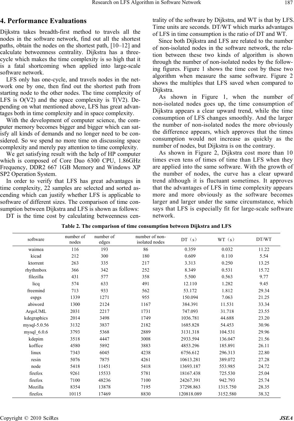

Research on LFS Algorithm in Software Network 187
4. Performance Evaluations
Dijkstra takes breadth-first method to travels all the
nodes in the software network, find out all the shortest
paths, obtain the nodes on the shortest path, [10–12] and
calculate betweenness centrality. Dijkstra has a three-
cycle which makes the time complexity is so high that it
is a fatal shortcoming when applied into large-scale
software network.
LFS only has one-cycle, and travels nodes in the net-
work one by one, then find out the shortest path from
starting node to the other nodes. The time complexity of
LFS is O(V2) and the space complexity is T(V2). De-
pending on what mentioned above, LFS has great advan-
tages both in time complexity and in space complexity.
With the development of computer science, the com-
puter memory becomes bigger and bigger which can sat-
isfy all kinds of demands and no longer need to be con-
sidered. So we spend no more time on discussing space
complexity and merely pay attention to time complexity.
We get satisfying result with the help of HP computer
which is composed of Core Duo 6300 CPU, 1.86GHz
Frequency, DDR2 667 1GB Memory and Windows XP
SP2 Operation System.
In order to verify that LFS has great advantages in
time complexity, 22 samples are selected and sorted as-
cending which can justify whether LFS is applicable to
software of different sizes. The comparison of time con-
sumption between Dijkstra and LFS is shown as follows:
DT is the time cost by calculating betweenness cen-
trality of the software by Dijkstra, and WT is that by LFS.
Time units are seconds. DT/WT which marks advantages
of LFS in time consumption is the ratio of DT and WT.
Since both Dijkstra and LFS are related to the number
of non-isolated nodes in the software network, the rela-
tion between these two kinds of algorithm is shown
through the number of non-isolated nodes by the follow-
ing figures. Figure 1 shows the time cost by these two
algorithm when measure the same software. Figure 2
shows the multiples that LFS saved when compared to
Dijkstra.
As shown in Figure 1, when the number of
non-isolated nodes goes up, the time consumption of
Dijkstra appears a clear upward trend, while the time
consumption of LFS changes smoothly. And the larger
the number of non-isolated nodes the more obviously
the difference appears, which approves that the times
consumption would not increase as quickly as the
number of nodes, but Dijkstra is on the contrary.
As shown in Figure 2, Dijkstra cost more than 10
times even tens of times of time than LFS when they
are applied into the same software. With the growth of
the number of nodes, the curve has a clear upward
trend although it is fluctuant sometimes. It approves
that the advantages of LFS in time complexity appears
more and more obviously as the software becomes
larger and larger under the same circumstance, which
says that LFS is especially fit for large-scale software
network.
Table 2. The comparison of time consumption betw ee n Dijkstra and LFS
software number of
nodes number of edges number of non- isolated nodes DT（s） WT（s） DT/WT
waimea 116 193 86 0.359 0.032 11.22
kicad 212 300 180 0.609 0.110 5.54
ktorrent 263 335 217 3.313 0.250 13.25
rhythmbox 366 342 252 8.349 0.531 15.72
filezilla 431 577 358 5.500 0.563 9.77
licq 574 633 491 12.110 1.282 9.45
freemind 713 933 562 53.172 1.812 29.34
espgs 1339 1271 955 150.094 7.063 21.25
abiword 1300 2124 1167 384.391 11.531 33.34
ArgoUML 2031 2217 1731 747.093 31.718 23.55
kdegraphics 2014 3498 1749 1036.781 44.688 23.20
mysql-5.0.56 3132 3837 2182 1685.828 54.453 30.96
mysql_6.0.6 3793 5368 2889 3131.318 104.531 29.96
kdepim 3518 4447 3008 2933.594 136.047 21.56
koffice 4580 5892 3883 4853.296 185.891 26.11
linux 7343 6045 4238 6756.612 296.313 22.80
resin 5076 7875 4261 10613.281 389.072 27.28
node 5418 11451 5418 13693.187 553.985 24.72
firefox 9261 15533 5781 18167.438 725.530 25.04
firefox 7100 48236 7100 24267.391 942.793 25.74
Mozilla 8354 13878 7195 37298.863 1315.750 28.35
firefox 10115 17469 8830 120818.089 3152.580 38.32

Research on LFS Algorithm in Software Network 188
Figure 1. The time cost by Dijkstra and LFS
Figure 2. The multiples that LFS saved when compared to Dijkstra
As shown in Figure 2, the value of DT/WT shows an
upward trend in volatility. Due to the relationship be-
tween the time complexity of LFS algorithm and the
complexity of the network itself, the value of DT/WT
depends on the size of the network which is equals to
the sum of the length of the entire shortest path. When

Research on LFS Algorithm in Software Network 189
the software network is a little more complex and the
lengths of shortest paths between some nodes are rela-
tive longer, LFS algorithm’s time complexity will in-
crease. For the same reason, when a more uniform dis-
tribution of the network and the lengths of shortest
paths between some nodes are relative shorter, the ad-
vantage of LFS is fully reflected that the time com-
plexity of LFS drops to relative small and the time
consumption comes down too, but Dijkstra doesn’t
have such feature. Therefore, the value of DT/WT
shows an upward trend in volatility. However, the
curve appears an upward trend from the whole.
As mentioned above, the low time complexity of
LFS can meet the needs of starting research on
large-scale software and solve the problems brought by
time complexity in the software measurement. At the
same time, the accurate data obtained will bring accu-
rate and reliable conclusion in practical research work.
5 Conclusions
LFS can solve a series of problems brought by the tra-
ditional algorithm. It has advantages both in time com-
plexity and accuracy which are so important in practi-
cal research work that may result in disaster conclusion
without it. LFS improve the efficiency and the accu-
racy to calculate the betweenness centrality, which
ensures the further research to be continued smoothly.
REFERENCES
[1] M. Pióro, A. Szentesi, J. Harmatos, A. Juttner, P. Ga-
jowniczek, and S. Kozdrowski, “On open shortest path
first related network optimization problems,” Perform-
ance Evaluation, Vol. 48, pp. 201–223, May 2002.
[2] E. P. F. Chan and N. Zhang, “Finding shortest paths in
large network systems,” Proceedings of the 9th ACM In-
ternational Workshop on Advances in Geographic Infor-
mation Systems (ACMGIS2001), Atlanta, Georgia, pp.
160–166, 2001.
[3] D. Awduchen, A. Chiu, A. Elwalid, I. Widjaja, and X.
Xiao, “Overview and principles of internet traffic engi-
neering,” RFC 3272, May 2002.
[4] D. Torrieri, “Algorithms for finding an optimal set of
short disjoint paths in a communication network,” Com-
munications, IEEE Transactions, Vol. 40, No. 11, pp.
1698–1702, 1992.
[5] B. Fortz and M. Thorup, “Internet traffic engineering by
optimizing OSPF weights,” in Proceedings IEEE INFO-
COM, pp. 519–528, 2000.
[6] X. Zhang, H. Zhao, W. B. Zhang, and C. Li, “Research on
CFR algorithm for Internet,” Journal on Communications,
Vol. 27, No. 9, September 2006.
[7] B. Fortz and M. Thorup, “Optimizing OSPF/IS-IS
weights in a changing world,” IEEE Journal on Selected
Areas in Communications, Vol. 20, No. 5, pp. 756–767,
May 2002.
[8] G. Rétvári and T. Cinkler, “Practical OSPF traffic engi-
neering,” IEEE Communications Letters, Vol. 8, No. 11,
pp. 689–691, November 2004.
[9] A. R. Soltani, H. Tawfik, J. Y .Goulermas, et al., “Path
planning in construction sites: Performance evaluation of
the dijkstra, a* and GA search algorithms,” Advanced
Engineering Informatics, Vol. 16, No. 4, pp. 291–303,
2002.
[10] Z. Wang, “Internet QoS: Architectures and mechanisms
for quality of service,” Academic Press, CA, San Diego,
2001.
[11] M. Pióro and D. Medhi, “Routing, flow, and capacity
design in communication and computer networks,” Mor-
gan Kaufmann, CA, San Diego, November 2004.
[12] W. Ben-Ameur and E. Gourdin, “Internet routing and
related topology issues,” SIAM Journal on Discrete
Mathematics, Vol. 17, No. 1, pp. 18–49, 2003.
[13] Gamma Erich, Helm Richard, Johnson Ralph, and Vlis-
sides John, “Design patterns: Elements of reusable ob-
ject-oriented software,” Addison-Wesley Longman Pub-
lishing Co., Inc. Boston, USA, 1995.
[14] M. M. Lehma and J. F. Rmail, “Software evolution and
software evolution processes,” Annals of Software Engi-
neering, Vol. 14, No. 1, pp. 275–309, 2002.
[15] B. Dougherty, J. White, C. Thompson, and D. C. Schmidt,
“Automating hardware and software evolution analysis,”
Engineering of Computer Based Systems (ECBS), 16th
Annual IEEE International Conference and Workshop on
the[C], pp. 265–274, 2009.
[16] S. N. Dorogovtsev and J. F. Mendes, “Scaling properties
of scale-free evolving networks: Continuous approach,”
Physical Review E, Vol. 63, No. 5, pp. 56125, 2001.
[17] N. Zhao, T. Li, L. L. Yang, Y. Yu, F. Dai, and W. Zhang,
“The resource optimization of software evolution proc-
esses,” Advanced Computer Control International Con-
ference on [C] (ICACC), pp. 332–336, 2009.
[18] B. Behm, “Some future trends and implications for sys-
tems and software engineering processes,” Systems En-
gineering, Vol. 9, No. 1, pp. 1–19, 2006.
[19] Lollini Paolo, Bondavalli Andrea, and Di Giandomenico
Felicita, “A decomposition-based modeling framework
for complex systems,” IEEE Transaction on Reliability,
Vol. 58, No. 1, pp. 20–33, 2009.
[20] Y. Ma and K. He, “A complexity metrics set for
large-scale object-oriented software systems,” in Pro-
ceedings of 6th International Conference on Computer
and Information Technology, pp. 189–189, 2006.
[21] K. Madhavi and A. A. Rao, “A framework for visualizing
model-driven software evolution,” IEEE International
Advance Computing Conference (IACC), pp. 1628–1633,
2009.
[22] S. Valverde and R. V. Sole, “Network notifs in computa-
tional graphs: A case study in software architecture,”
Physical Review E, Vol. 72, No. 2, pp. 26107, 2005.