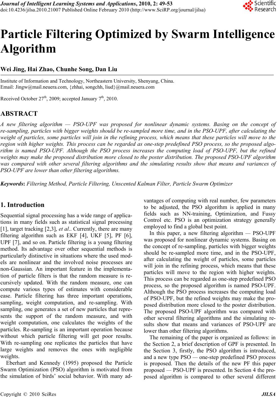Journal of Intelligent Learning Systems and Applications, 2010, 2: 49-53
doi:10.4236/jilsa.2010.21007 Published Online February 2010 (http://www.SciRP.org/journal/jilsa)
Particle Filtering Optimized by Swarm Intelligence
Algorithm
Wei Jing, Hai Zhao, Chunhe Song, Dan Liu
Institute of Information and Technology, Northeastern University, Shenyang, China.
Received October 27th, 2009; accepted January 7th, 2010.
ABSTRACT
A new filtering algorithm — PSO-UPF was proposed for nonlinear dynamic systems. Basing on the concept of
re-sampling, particles with bigger weights should be re-sampled more time, and in the PSO-UPF, after calculating the
weight of particles, some particles will join in the refining process, which means that these particles will move to the
region with higher weights. This process can be regarded as one-step predefined PSO process, so the proposed algo-
rithm is named PSO-UPF. Although the PSO process increases the computing load of PSO-UPF, but the refined
weights may make the proposed distribution more closed to the poster distribution. The proposed PSO-UPF algorithm
was compared with other several filtering algorithms and the simulating results show that means and variances of
PSO-UPF are lower than other filtering algorithms.
Keywords: Filtering Method, Particle Filtering, Unscented Kalman Filter, Particle Swarm Optimizer
1. Introduction
Sequential signal processing has a wide range of applica-
tions in many fields such as statistical signal processing
[1], target tracking [2,3], et al.. Currently, there are many
filtering algorithm such as EKF [4], UKF [5], PF [6],
UPF [7], and so on. Particle filtering is a young filtering
method. Its advantage over other sequential methods is
particularly distinctive in situations where the used mod-
els are nonlinear and the involved noise processes are
non-Gaussian. An important feature in the implementa-
tion of particle filters is that the random measure is re-
cursively updated. With the random measure, one can
compute various types of estimates with considerable
ease. Particle filtering has three important operations,
sampling, weight computation, and re-sampling. With
sampling, one generates a set of new particles that repre-
sents the support of the random measure, and with
weight computation, one calculates the weights of the
particles. Re-sampling is an important operation because
without which particle filtering will get poor results.
With re-sampling one replicates the particles that have
large weights and removes the ones with negligible
weights.
Eberhart and Kennedy (1995) proposed the Particle
Swarm Optimization (PSO) algorithm is motivated from
the simulation of birds’ social behavior. With many ad-
vantages of computing with real number, few parameters
to be adjusted, the PSO algorithm is applied in many
fields such as NN-training, Optimization, and Fussy
Control etc. PSO is an optimization strategy generally
employed to find a global best point.
In this paper, a new filtering algorithm — PSO-UPF
was proposed for nonlinear dynamic systems. Basing on
the concept of re-sampling, particles with bigger weights
should be re-sampled more time, and in the PSO-UPF,
after calculating the weight of particles, some particles
will join in the refining process, which means that these
particles will move to the region with higher weights.
This process can be regarded as one-step predefined PSO
process, so the proposed algorithm is named PSO-UPF.
Although the PSO process increases the computing load
of PSO-UPF, but the refined weights may make the pro-
posed distribution more closed to the poster distribution.
The proposed PSO-UPF algorithm was compared with
other several filtering algorithms and the simulating re-
sults show that means and variances of PSO-UPF are
lower than other filtering algorithms.
The remaining of the paper is organized as follows: in
the Section 2, a brief description of GPF is presented. In
the Section 3, firstly, the PSO algorithm is introduced,
and a new type PSO — one-step predefined PSO process
is proposed. Then the details of the new PF this paper
proposed — PSO-UPF is presented. In Section 4 the pro-
posed algorithm is compared to other several different

Particle Filtering Optimized by Swarm Intelligence Algorithm 50
filtering algorithms, and finally, some concluding re-
marks is given in Section 5.
2. Basic Particle Filter
The problem being addressed here is an estimating prob-
lem of the state of a system as a set of observations be-
comes available on-line, which can be expressed as fol-
lows:
1
()
(,)
tt
ttt
1t
t
x
fx w
yhux v




x
n
(1)
where ,,, are the state
of the system, the output observations, the input observa-
tions, the process noise and the measurement noise. The
mappings:
x
n
t
x y
n
t
y u
n
t
u v
n
t
v
:*
xx
nn
f and represent the
deterministic process and measurement models.
:* y
xv n
nn
h 
In the bayes filtering paradigm, the posterior distribu-
tion is updated recursively over the current state t
x
given all observations up to and including
time as follows [6]:
1
{}
t
tii
Zz


t
111
(| )(|)(| )
ttttt tk1
p
xYpxxpxY dx


(2)
1
1
(|)(|)
(|) (| )
tt tt
tt
tt
p
yxpxY
px Ypy Y


 (3)
1
1
(|)(|)
(|) (| )
tt tt
tt
tt
p
yxpxY
px Ypy Y


 (4)
Using Monte Carlo sampling points, particle filter exe-
cutes the filtering process by generating weighted sam-
pling points of state variances recursively. Generic parti-
cle filter algorithm can be predicted as follows [6]:
Initialization
For each particle
draw the states()
0
i
x
from the prior;
0
()px
End
For each loop
importance sampling step
For each particle
sample ()()
00:1
ˆ~( |,)
ii
tt t 1:
x
qx xy

End
For each particle
evaluate the importance weights up to a normalizing
constant:
()() ()
() ()1
1() ()
0: 11:
ˆ
(| )( |)
ˆˆ (| ,)
iii
ii
ttt t
tt ii
ttt
py xpxx
ww qx xy



 (5)
For each particle, normalize the importance weights:
()()( )1
1
1
[
N
ii j
tt t
j
ww w





// Re-sample
Eliminate the samples with low importance weights
and multiply the samples with high importance weights,
to obtain N random samples ()
0:
i
k
x
approximately distrib-
uted according to .
0: 1:
(|
kk
pxz )
Assign each particle an equal weight: . 1/
i
t
wN
When executing particle filtering, the choice of the
proposal distribution is very important. Usually, the tran-
sition prior distribution is chosen to be the proposal dis-
tribution:
1
(|,) (| )
ttt tk
qxXYpx x

1
(7)
But as not considering the recent observation, when
using the transition prior distribution as the proposal dis-
tribution, the filtering result is usually poor, especially
when the noise is heavy. In this paper, a kind of
semi-iterative unscented transformation was proposed to
address this issue.
3. The PSO-UPF Algorithm
3.1 Particle Swarm Optimizer Algorithm
PSO is an optimization strategy generally employed to
find a global best point. At each time step, a particle up-
dates its position and velocity by the following equa-
tions:
11
22
(1)* ()()(()())
()( ()())
ijijj ijij
jgj ij
vtwvt crtptxt
crtptx t
 
 (8)
(1)() (1)
ijij ij
xtxt vt

 (9)
maxmax min
max
()
g
t
t
wwww  (10)
where {1, 2,...,}jDn

,{1, 2,...,}in

,n is the size of the
population andis the Dimension of the space
searched; is the inertia weight, generally updated as
equation 3 [10], and is the maximal evolution gen-
erations. and are two positive constants; and
are two random values into the range
Dn
w
g
1
c2 c
max
1
r
2
r


0, 1.
3.2 PSO in the PF Process
As depicted in the Section 2, in the re-sampling process
of regular particle filtering, the particles with bigger
weights will have more offspring, while the particles
with smaller weights will have few or even on offspring.
It inspires us to find more particles with big weights and
reduce the number of particles with small weights, which
will make the proposal distribution more closed to the
poster distribution. And it is the aim of using particles
swarm optimization in the particles filtering process.
] (6) The most important issue of using particles swarm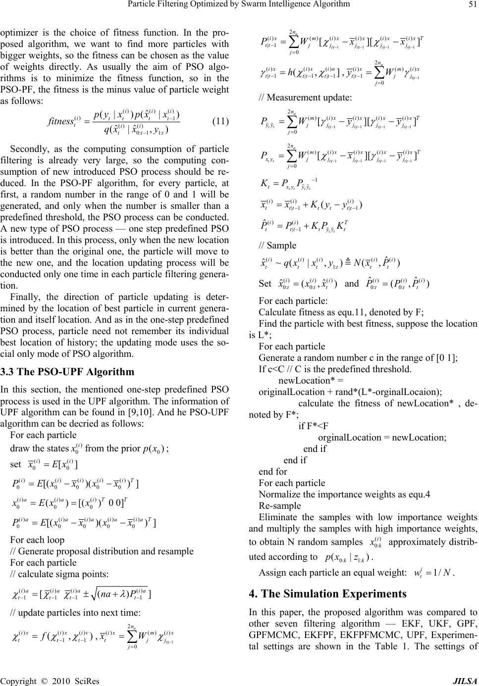

Particle Filtering Optimized by Swarm Intelligence Algorithm51
optimizer is the choice of fitness function. In the pro-
posed algorithm, we want to find more particles with
bigger weights, so the fitness can be chosen as the value
of weights directly. As usually the aim of PSO algo-
rithms is to minimize the fitness function, so in the
PSO-PF, the fitness is the minus value of particle weight
as follows:
()() ()
() 1
() ()
0: 11:
ˆ
(| )( |)
ˆˆ (| ,)
iii
ittt t
tii
ttt
py xpxx
fitness qxxy


 (11)
Secondly, as the computing consumption of particle
filtering is already very large, so the computing con-
sumption of new introduced PSO process should be re-
duced. In the PSO-PF algorithm, for every particle, at
first, a random number in the range of 0 and 1 will be
generated, and only when the number is smaller than a
predefined threshold, the PSO process can be conducted.
A new type of PSO process — one step predefined PSO
is introduced. In this process, only when the new location
is better than the original one, the particle will move to
the new one, and the location updating process will be
conducted only one time in each particle filtering genera-
tion.
Finally, the direction of particle updating is deter-
mined by the location of best particle in current genera-
tion and itself location. And as in the one-step predefined
PSO process, particle need not remember its individual
best location of history; the updating mode uses the so-
cial only mode of PSO algorithm.
3.3 The PSO-UPF Algorithm
In this section, the mentioned one-step predefined PSO
process is used in the UPF algorithm. The information of
UPF algorithm can be found in [9,10]. And he PSO-UPF
algorithm can be decried as follows:
For each particle
draw the states()
0
i
x
from the prior;
0
()px
set () ()
00
[]
ii
x
Ex
()()() ()()
00000
[( )()]
iiiii
P Exxxx 
T
()() ()
000
()[()00]
iaiai TT
xExx
()()() ()()
00000
[()() ]
iaiaiaiaiaT
PExxxx 
For each loop
// Generate proposal distribution and resample
For each particle
// calculate sigma points:
()() ()()
111 1
[()
iaiaiaia
ttt t
na P  
 
]
// update particles into next time:
()() ()
11
(,
ixix iv
ttt
f 

),|1
2
()( )()
0
a
tt
n
ixm ix
tj
j
xW
|1 |1 |1 |1
2
()()() ()() ()
|1
0
[][]
a
tt tt tt tt
n
ix mixixixix
ttjjjjj
j
PW xx 




T
()() ()
|1|1 |1
(,
ixix in
tttttt
h 

]

,|1
2
()( )()
|1
0
a
tt
n
ixm ix
ttjj
j
yW





// Measurement update:
|1 |1|1 |1
2
()() ()() ()
0
[][]
a
tttt tttt tt
n
mixixixix
yyjj jj j
j
PW yy 



 
T
|1|1 |1|1
2
( )()()()()
0
[][
a
t ttttttttt
n
mix ixix ixT
xyj jjjj
j
PW xy 
 


]
1
tt tt
txyyy
KPP


() ()()
|1 |1
()
ii i
ttttttt
xx Kyy


() ()
|1
ˆ
tt
ii
ttttyy
PP KPK



T
t
// Sample
()()()() ()
1: ˆ
ˆ~(|, )(,)
iiii
tttttt
i
x
qxx yNx P
Set ()() ()
0: 0:
ˆ
(,)
iii
ttt
ˆ
x
xx and
()() ()
0: 0:
ˆˆ
(,
ii
ttt
PPP)
i
For each particle:
Calculate fitness as equ.11, denoted by F;
Find the particle with best fitness, suppose the location
is L*;
For each particle
Generate a random number c in the range of [0 1];
If c<C // C is the predefined threshold.
newLocation* =
originalLocation + rand*(L*-orginalLocaion);
calculate the fitness of newLocation* , de-
noted by F*;
if F*<F
orginalLocation = newLocation;
end if
end if
end for
For each particle
Normalize the importance weights as equ.4
Re-sample
Eliminate the samples with low importance weights
and multiply the samples with high importance weights,
to obtain N random samples ()
0:
i
k
x
approximately distrib-
uted according to .
0: 1:
(|
kk
pxz )
Assign each particle an equal weight: . 1/
i
t
wN
4. The Simulation Experiments
In this paper, the proposed algorithm was compared to
other seven filtering algorithm — EKF, UKF, GPF,
GPFMCMC, EKFPF, EKFPFMCMC, UPF, Experimen-
tal settings are shown in the Table 1. The settings of
j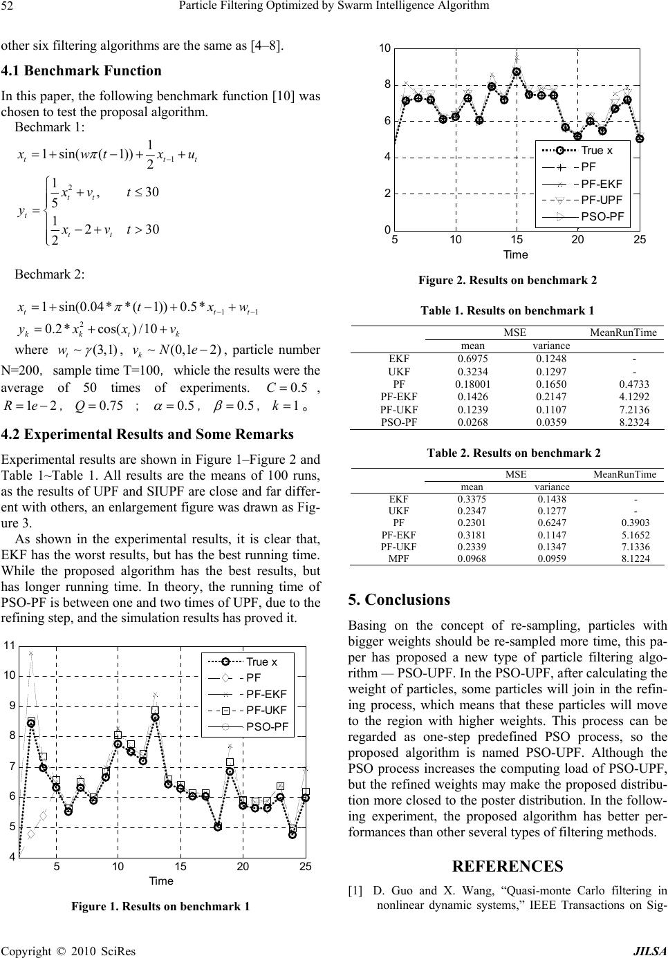





Particle Filtering Optimized by Swarm Intelligence Algorithm 52
other six filtering algorithms are the same as [4–8].
4.1 Benchmark Function
In this paper, the following benchmark function [10] was
chosen to test the proposal algorithm.
Bechmark 1:
1
2
1
1sin((1)) 2
1,30
5
1230
2
tt
tt
t
tt
t
x
wtx u
xv t
y
xvt


 




 


Bechmark 2:
11
1 sin(0.04**(1))0.5*
ttt
x
txw



2
0.2*cos()/10
kkt
yxx 
k
v
where ~(3,1)
t
w

, , particle number
N=200，sample time T=100，whicle the results were the
average of 50 times of experiments.
~(0,1 2)
k
vNe
0.5C

,
， ； 1Re20.75Q0.5


，0.5

，1k

。
4.2 Experimental Results and Some Remarks
Experimental results are shown in Figure 1–Figure 2 and
Table 1~Table 1. All results are the means of 100 runs,
as the results of UPF and SIUPF are close and far differ-
ent with others, an enlargement figure was drawn as Fig-
ure 3.
As shown in the experimental results, it is clear that,
EKF has the worst results, but has the best running time.
While the proposed algorithm has the best results, but
has longer running time. In theory, the running time of
PSO-PF is between one and two times of UPF, due to the
refining step, and the simulation results has proved it.
510 15 20 25
4
5
6
7
8
9
10
11
Time
True x
PF
PF-EKF
PF-UKF
PSO-PF
Figure 1. Results on benchmark 1
510 1520 25
0
2
4
6
8
10
Time
True x
PF
PF-EKF
PF-UPF
PSO-PF
Figure 2. Results on benchmark 2
Table 1. Results on benchmark 1
MSE MeanRunTime
mean variance
EKF 0.69750.1248 -
UKF 0.3234 0.1297 -
PF 0.180010.1650 0.4733
PF-EKF0.14260.2147 4.1292
PF-UKF0.12390.1107 7.2136
PSO-PF0.02680.0359 8.2324
Table 2. Results on benchmark 2
MSE MeanRunTime
mean variance
EKF 0.3375 0.1438 -
UKF 0.2347 0.1277 -
PF 0.2301 0.6247 0.3903
PF-EKF0.3181 0.1147 5.1652
PF-UKF0.2339 0.1347 7.1336
MPF 0.0968 0.0959 8.1224
5. Conclusions
Basing on the concept of re-sampling, particles with
bigger weights should be re-sampled more time, this pa-
per has proposed a new type of particle filtering algo-
rithm — PSO-UPF. In the PSO-UPF, after calculating the
weight of particles, some particles will join in the refin-
ing process, which means that these particles will move
to the region with higher weights. This process can be
regarded as one-step predefined PSO process, so the
proposed algorithm is named PSO-UPF. Although the
PSO process increases the computing load of PSO-UPF,
but the refined weights may make the proposed distribu-
tion more closed to the poster distribution. In the follow-
ing experiment, the proposed algorithm has better per-
formances than other several types of filtering methods.
REFERENCES
[1] D. Guo and X. Wang, “Quasi-monte Carlo filtering in
nonlinear dynamic systems,” IEEE Transactions on Sig-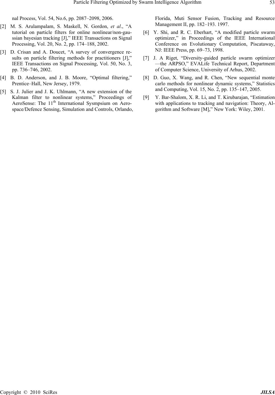

Particle Filtering Optimized by Swarm Intelligence Algorithm 53
nal Process, Vol. 54, No.6, pp. 2087–2098, 2006.
[2] M. S. Arulampalam, S. Maskell, N. Gordon, et al., “A
tutorial on particle filters for online nonlinear/non-gau-
ssian bayesian tracking [J],” IEEE Transactions on Signal
Processing, Vol. 20, No. 2, pp. 174–188, 2002.
[3] D. Crisan and A. Doucet, “A survey of convergence re-
sults on particle filtering methods for practitioners [J],”
IEEE Transactions on Signal Processing, Vol. 50, No. 3,
pp. 736–746, 2002.
[4] B. D. Anderson, and J. B. Moore, “Optimal filtering,”
Prentice–Hall, New Jersey, 1979.
[5] S. J. Julier and J. K. Uhlmann, “A new extension of the
Kalman filter to nonlinear systems,” Proceedings of
AeroSense: The 11th International Sysmpsium on Aero-
space/Defence Sensing, Simulation and Controls, Orlando,
Florida, Muti Sensor Fusion, Tracking and Resource
Management II, pp. 182–193. 1997.
[6] Y. Shi, and R. C. Eberhart, “A modified particle swarm
optimizer,” in Proceedings of the IEEE International
Conference on Evolutionary Computation, Piscataway,
NJ: IEEE Press, pp. 69–73, 1998.
[7] J. A Riget, “Diversity-guided particle swarm optimizer
—the ARPSO,” EVALife Technical Report, Department
of Computer Science, University of Arhus, 2002.
[8] D. Guo, X. Wang, and R. Chen, “New sequential monte
carlo methods for nonlinear dynamic systems,” Statistics
and Computing, Vol. 15, No. 2, pp. 135–147, 2005.
[9] Y. Bar-Shalom, X. R. Li, and T. Kirubarajan, “Estimation
with applications to tracking and navigation: Theory, Al-
gorithm and Software [M],” New York: Wiley, 2001.