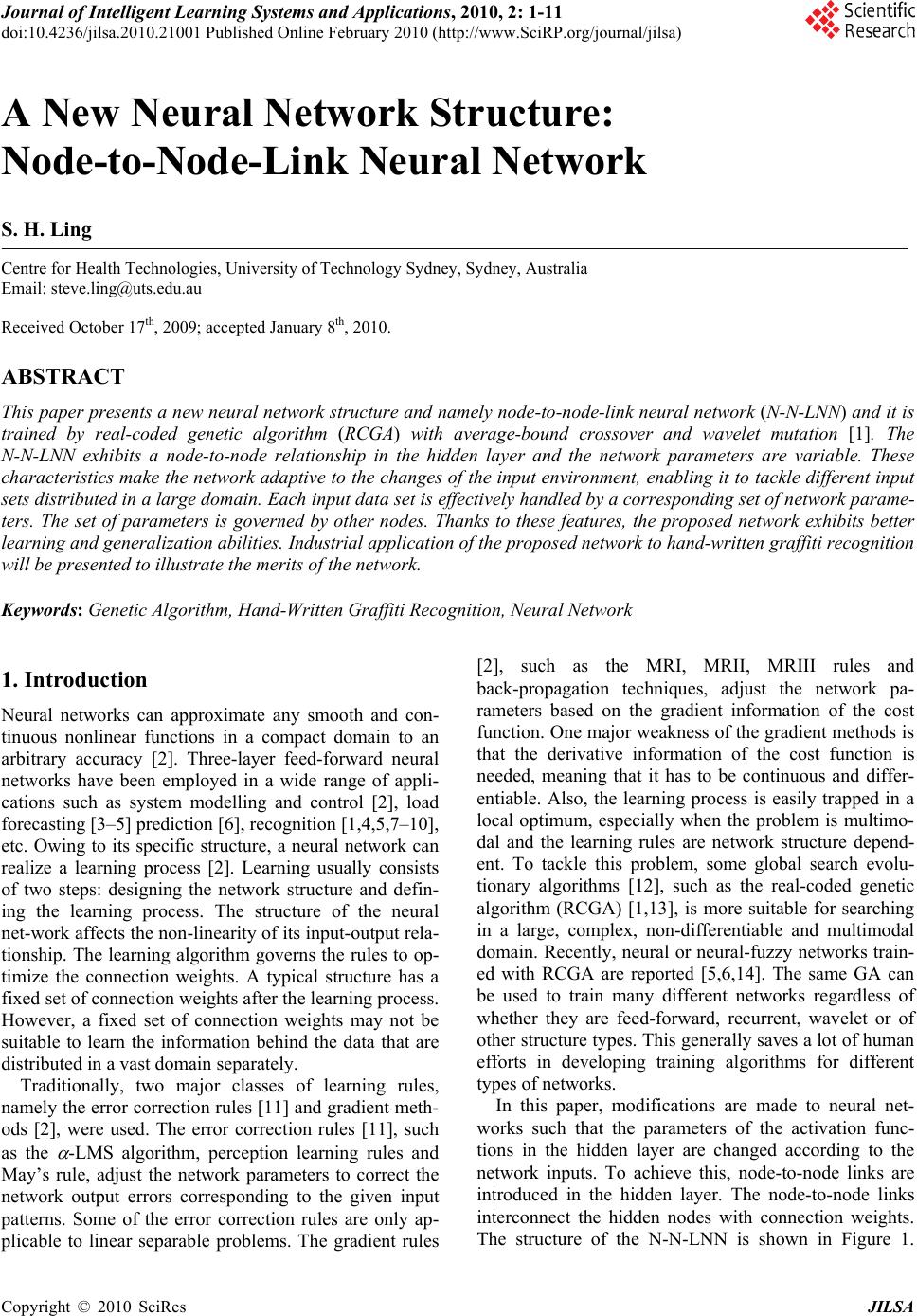Journal of Intelligent Learning Systems and Applications, 2010, 2: 1-11
doi:10.4236/jilsa.2010.21001 Published Online February 2010 (http://www.SciRP.org/journal/jilsa)
1
A New Neural Network Structure:
Node-to-Node-Link Neural Network
S. H. Ling
Centre for Health Technologies, University of Technology Sydney, Sydney, Australia
Received October 17th, 2009; accepted January 8th, 2010.
ABSTRACT
This paper presents a new neural network structure and namely node-to-node-link neural network (N-N-LNN) and it is
trained by real-coded genetic algorithm (RCGA) with average-bound crossover and wavelet mutation [1]. The
N-N-LNN exhibits a node-to-node relationship in the hidden layer and the network parameters are variable. These
characteristics make the network adaptive to the changes of the input environment, enabling it to tackle different input
sets distributed in a large domain. Each input data set is effectively handled by a corresponding set of network parame-
ters. The set of parameters is governed by other nodes. Thanks to these features, the proposed network exhibits better
learning and generalization abilities. Industrial application of the proposed network to hand-written graffiti recognition
will be presented to illustrate the merits of the network.
Keywords: Genetic Algorithm, Hand-Written Graffiti Recognition, Neural Network
1. Introduction
Neural networks can approximate any smooth and con-
tinuous nonlinear functions in a compact domain to an
arbitrary accuracy [2]. Three-layer feed-forward neural
networks have been employed in a wide range of appli-
cations such as system modelling and control [2], load
forecasting [3–5] prediction [6], recognition [1,4,5,7–10],
etc. Owing to its specific structure, a neural network can
realize a learning process [2]. Learning usually consists
of two steps: designing the network structure and defin-
ing the learning process. The structure of the neural
net-work affects the non-linearity of its input-output rela-
tionship. The learning algorithm governs the rules to op-
timize the connection weights. A typical structure has a
fixed set of connection weights after the learning process.
However, a fixed set of connection weights may not be
suitable to learn the information behind the data that are
distributed in a vast domain separately.
Traditionally, two major classes of learning rules,
namely the error correction rules [11] and gradient meth-
ods [2], were used. The error correction rules [11], such
as the
 -LMS algorithm, perception learning rules and
May’s rule, adjust the network parameters to correct the
network output errors corresponding to the given input
patterns. Some of the error correction rules are only ap-
plicable to linear separable problems. The gradient rules
[2], such as the MRI, MRII, MRIII rules and
back-propagation techniques, adjust the network pa-
rameters based on the gradient information of the cost
function. One major weakness of the gradient methods is
that the derivative information of the cost function is
needed, meaning that it has to be continuous and differ-
entiable. Also, the learning process is easily trapped in a
local optimum, especially when the problem is multimo-
dal and the learning rules are network structure depend-
ent. To tackle this problem, some global search evolu-
tionary algorithms [12], such as the real-coded genetic
algorithm (RCGA) [1,13], is more suitable for searching
in a large, complex, non-differentiable and multimodal
domain. Recently, neural or neural-fuzzy networks train-
ed with RCGA are reported [5,6,14]. The same GA can
be used to train many different networks regardless of
whether they are feed-forward, recurrent, wavelet or of
other structure types. This generally saves a lot of human
efforts in developing training algorithms for different
types of networks.
In this paper, modifications are made to neural net-
works such that the parameters of the activation func-
tions in the hidden layer are changed according to the
network inputs. To achieve this, node-to-node links are
introduced in the hidden layer. The node-to-node links
interconnect the hidden nodes with connection weights.
The structure of the N-N-LNN is shown in Figure 1.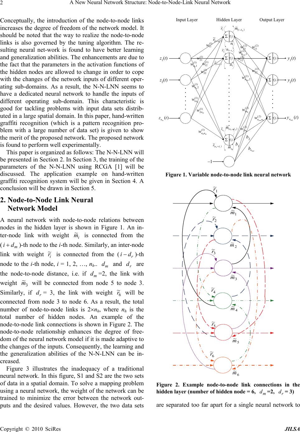

A New Neural Network Structure: Node-to-Node-Link Neural Network 2
Conceptually, the introduction of the node-to-node links
increases the degree of freedom of the network model. It
should be noted that the way to realize the node-to-node
links is also governed by the tuning algorithm. The re-
sulting neural net-work is found to have better learning
and generalization abilities. The enhancements are due to
the fact that the parameters in the activation functions of
the hidden nodes are allowed to change in order to cope
with the changes of the network inputs of different oper-
ating sub-domains. As a result, the N-N-LNN seems to
have a dedicated neural network to handle the inputs of
different operating sub-domain. This characteristic is
good for tackling problems with input data sets distrib-
uted in a large spatial domain. In this paper, hand-written
graffiti recognition (which is a pattern recognition pro-
blem with a large number of data set) is given to show
the merit of the proposed network. The proposed network
is found to perform well experimentally.
This paper is organized as follows: The N-N-LNN will
be presented in Section 2. In Section 3, the training of the
parameters of the N-N-LNN using RCGA [1] will be
discussed. The application example on hand-written
graffiti recognition system will be given in Section 4. A
conclusion will be drawn in Section 5.
2. Node-to-Node Link Neural
Network Model
A neural network with node-to-node relations between
nodes in the hidden layer is shown in Figure 1. An in-
ter-node link with weight i
m
~
is connected from the
()-th node to the i-th node. Similarly, an inter-node
link with weight
m
di 
i
r
~
is connected from the (r di

)-th
node to the i-th node, i = 1, 2, …, nh.. and are
the node-to-node distance, i.e. if =2, the link with
weight
m
dr d
m
d
3
~
m will be connected from node 5 to node 3.
Similarly, if = 3, the link with weight
r
d6
~
r will be
connected from node 3 to node 6. As a result, the total
number of node-to-node links is 2nh, where nh is the
total number of hidden nodes. An example of the
node-to-node link connections is shown in Figure 2. The
node-to-node relationship enhances the degree of free-
dom of the neural network model if it is made adaptive to
the changes of the inputs. Consequently, the learning and
the generalization abilities of the N-N-LNN can be in-
creased.
Figure 3 illustrates the inadequacy of a traditional
neural network. In this figure, S1 and S2 are the two sets
of data in a spatial domain. To solve a mapping problem
using a neural network, the weight of the network can be
trained to minimize the error between the network out-
puts and the desired values. However, the two data sets
z1(t)
z2(t)
)(tz in
n


tf1(.)
tf1(.)
tf1(.)
tf2(.)
tf2(.)
tf2(.)
y1(t)
y2(t)
)(
t
yout
n
)1(
11
w
)1(
21
w
)1(
1
h
n
w)1(
12
w
)1(
22
w
)1(
2
h
n
w
)1(
inhnn
w
)1(
1in n
w
)1(
2in n
w
)2(
11
w
)2(
21
w
)2(
1
out
n
w
)2(
12
w
)2(
22
w
)2(
1h n
w
)2(
2h n
w
)2(
houtnn
w
Hidden LayerInput LayerOutput Layer
)2(
2
out
n
w
1
b1
b2
out
n
b
1
~
m
1
~
r

m
d
m1
~

r
d
r1
~
2
~
r

m
d
m2
~

r
d
r2
~
2
~
m
h
n
r
~

mhdn
m
~

rh dn
r
~
h
n
m
~
Figure 1. Variable node-to-node link neural network
2
~
m
4
~
m
5
~
m
6
~
m
1
~
m
3
~
m
1
~
r
2
~
r
3
~
r
4
~
r
5
~
r
6
~
r
Figure 2. Example node-to-node link connections in the
hidden layer (number of hidden node = 6, =2, = 3)
m
dr d
are separated too far apart for a single neural network to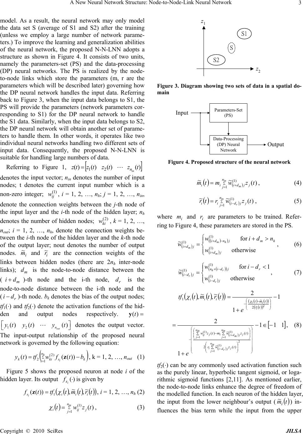

A New Neural Network Structure: Node-to-Node-Link Neural Network3

model. As a result, the neural network may only model
the data set S (average of S1 and S2) after the training
(unless we employ a large number of network parame-
ters.) To improve the learning and generalization abilities
of the neural network, the proposed N-N-LNN adopts a
structure as shown in Figure 4. It consists of two units,
namely the parameters-set (PS) and the data-processing
(DP) neural networks. The PS is realized by the node-
to-node links which store the parameters (m, r are the
parameters which will be described later) governing how
the DP neural network handles the input data. Referring
back to Figure 3, when the input data belongs to S1, the
PS will provide the parameters (network parameters cor-
responding to S1) for the DP neural network to handle
the S1 data. Similarly, when the input data belongs to S2,
the DP neural network will obtain another set of parame-
ters to handle them. In other words, it operates like two
individual neural networks handling two different sets of
input data. Consequently, the proposed N-N-LNN is
suitable for handling large numbers of data.
Referring to Figure 1,
denotes the input vector; nin denotes the number of input
nodes; t denotes the current input number which is a
non-zero integer; , i = 1, 2, …, nh; j = 1, 2, …, nin,
denote the connection weights between the j-th node of
the input layer and the i-th node of the hidden layer; nh
denotes the number of hidden nodes; , k = 1, 2, …,
nout; i = 1, 2, …, nh, denote the connection weights be-
tween the i-th node of the hidden layer and the k-th node
of the output layer; nout denotes the number of output
nodes.
 )()()()( 21 tztztztz in
n

)2(
ki
w
)1(
ij
w
i
m
~
and i r
~
are the connection weights of the
links between hidden nodes (there are 2nh inter-node
links); is the node-to-node distance between the
()-th node and the i-th node, is the
node-to-node distance between the i-th node and the
()-th node. bk denotes the bias of the output nodes;
tf1() and tf2() denote the activation functions of the hid-
den and output nodes respectively.
m
d
m
di 
r
di 
r
d
()t

y


denotes the output vector.
The input-output relationship of the proposed neural
network is governed by the following equation:
12
y()yt() ()t t


out
n
y




 h
i
n
ikskik btfwtfty 1
)2(
2))(()( z, k = 1, 2, …, nout (1)
Figure 5 shows the proposed neuron at node i of the
hidden layer. Its output is given by )(
i
s
f


 trtmttftfiiisi 
~
,
~
,))((1  z, i = 1, 2, …, nh (2)



in
n
jjiji tzwt 1
)1( )(
 , (3)
S2
S1
z1
z2
S
Figure 3. Diagram showing two sets of data in a spatial do-
main
Parameters-Set
(PS)
Data-Processing
(DP) Neural
Network
Input
Output
Figure 4. Proposed structure of the neural network




in
m
n
jjjdiii tzwmtm1
)1( )( ~~, (4)




in
r
n
jjjdiii tzwrtr 1
)1( )( ~~ , (5)
where and are parameters to be trained. Refer-
ring to Figure 4, these parameters are stored in the PS.
i
mi r
 









otherwise
for
~
)1(
)1(
)1(
jdi
hmjndi
jdi
m
hm
mw
ndiw
w, (6)
 









otherwise
1for
~
)1(
)1(
)1(
jdi
rjdin
jdi
r
rh
rw
diw
w, (7)







 trtmttf iii
~
~
,
1,

 

1
1
2
2 ~
2
~











tr
tmt
i
ii
e



 111
1
2
2
1
)1(
1
)1(
1
)1(
)(
~
2
)(
~
)(









































 
in
n
jj
j
r
di
i
in
n
jj
j
m
di
i
in
n
jj
ij
tzwr
tzwmtzw
e
 , (8)
tf2() can be any commonly used activation function such
as the purely linear, hyperbolic tangent sigmoid, or loga-
rithmic sigmoid functions [2,11]. As mentioned earlier,
the node-to-node links enhance the degree of freedom of
the modelled function. In each neuron of the hidden layer,
the input from the lower neighbour’s output (

 tmi
~
) in-
fluences the bias term while the input from the upper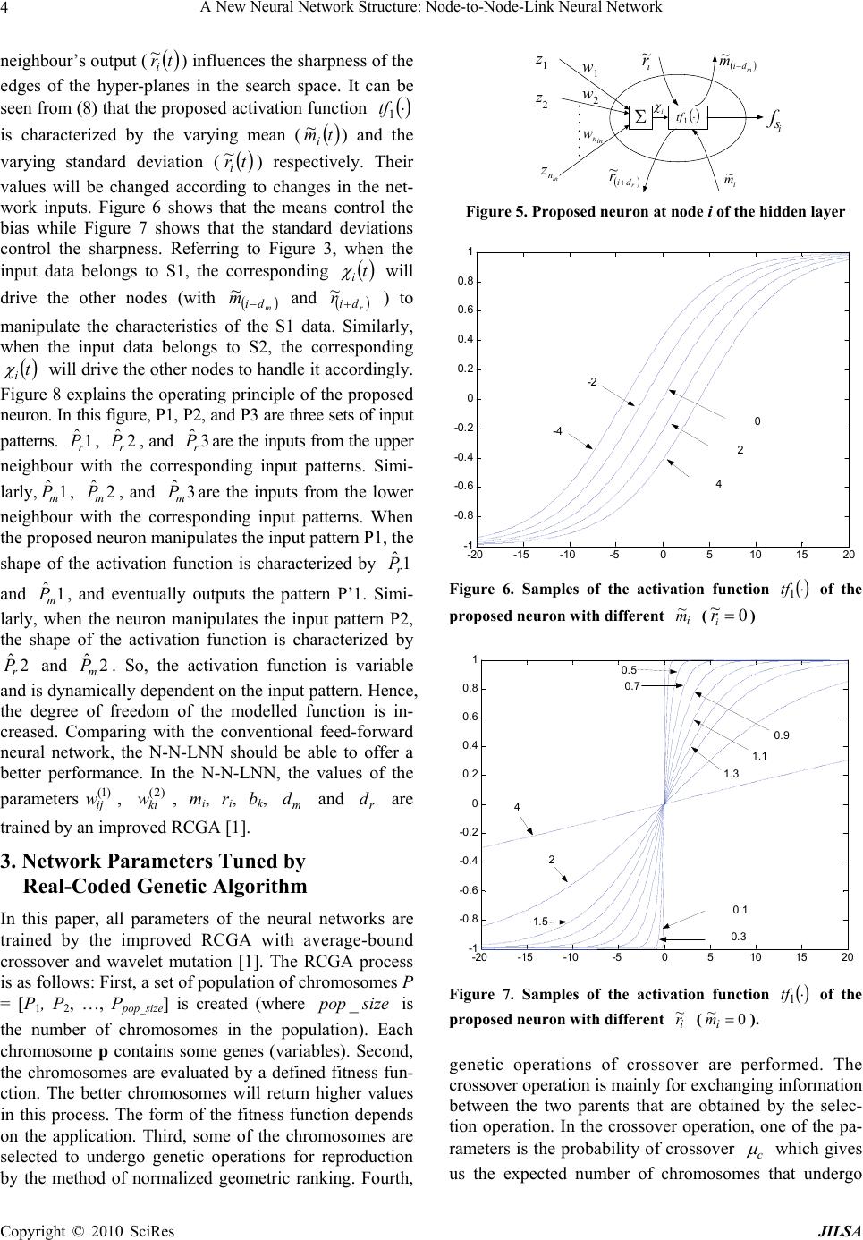

A New Neural Network Structure: Node-to-Node-Link Neural Network 4
neighbour’s output (

tri
~
) influences the sharpness of the
edges of the hyper-planes in the search space. It can be
seen from (8) that the proposed activation function



1
tf
is characterized by the varying mean (

tmi
~
) and the
varying standard deviation (

tri
~
) respectively. Their
values will be changed according to changes in the net-
work inputs. Figure 6 shows that the means control the
bias while Figure 7 shows that the standard deviations
control the sharpness. Referring to Figure 3, when the
input data belongs to S1, the corresponding

 t
i

will
drive the other nodes (with
 i
m

m
d
~
and

r
d  i
r
~
) to
manipulate the characteristics of the S1 data. Similarly,
when the input data belongs to S2, the corresponding
 t
i

will drive the other nodes to handle it accordingly.
Figure 8 explains the operating principle of the proposed
neuron. In this figure, P1, P2, and P3 are three sets of input
patterns. , , and are the inputs from the upper
neighbour with the corresponding input patterns. Simi-
larly, , , and are the inputs from the lower
neighbour with the corresponding input patterns. When
the proposed neuron manipulates the input pattern P1, the
shape of the activation function is characterized by
and , and eventually outputs the pattern P’1. Simi-
larly, when the neuron manipulates the input pattern P2,
the shape of the activation function is characterized by
and . So, the activation function is variable
and is dynamically dependent on the input pattern. Hence,
the degree of freedom of the modelled function is in-
creased. Comparing with the conventional feed-forward
neural network, the N-N-LNN should be able to offer a
better performance. In the N-N-LNN, the values of the
parameters , , mi, ri, bk, and are
trained by an improved RCGA [1].
1
ˆr
P
1ˆm P
1
ˆm
P
(
ij
w
2
ˆr
P
2
2
)1
3
ˆr
P
3
ˆm
P
ˆm
ˆm
P
)2(
ki
w
1
ˆr
P
r
size
P
2
ˆr
P
m
pop
d d
_
3. Network Parameters Tuned by
Real-Coded Genetic Algorithm
In this paper, all parameters of the neural networks are
trained by the improved RCGA with average-bound
crossover and wavelet mutation [1]. The RCGA process
is as follows: First, a set of population of chromosomes P
= [P1, P2, …, Ppop_size] is created (where is
the number of chromosomes in the population). Each
chromosome p contains some genes (variables). Second,
the chromosomes are evaluated by a defined fitness fun-
ction. The better chromosomes will return higher values
in this process. The form of the fitness function depends
on the application. Third, some of the chromosomes are
selected to undergo genetic operations for reproduction
by the method of normalized geometric ranking. Fourth,

z1
z2
w1
w2
i
r
~

r
di
r
~

m
di
m
~
i
m
~
i
s
f
 
1
tf
in
n
z
in
n
w
i

Figure 5. Proposed neuron at node i of the hidden layer
-20 -15 -10-505 10 1520
-1
-0.8
-0.6
-0.4
-0.2
0
0. 2
0. 4
0. 6
0. 8
1
0
2
4
-2
-4
Figure 6. Samples of the activation function



1
tf of the
proposed neuron with different i
m
~
(0
~

i
r)
-20 -15 -10 -5 0510 15 20
-1
-0.8
-0.6
-0.4
-0.2
0
0. 2
0. 4
0. 6
0. 8
1
4
2
1.5
1.3
1.1
0.9
0.7
0.5
0.3
0.1
Figure 7. Samples of the activation function



1
tf of the
proposed neuron with different ().
i
r
~0 ~
i
m
genetic operations of crossover are performed. The
crossover operation is mainly for exchanging information
between the two parents that are obtained by the selec-
tion operation. In the crossover operation, one of the pa-
rameters is the probability of crossover c

which gives
us the expected number of chromosomes that undergo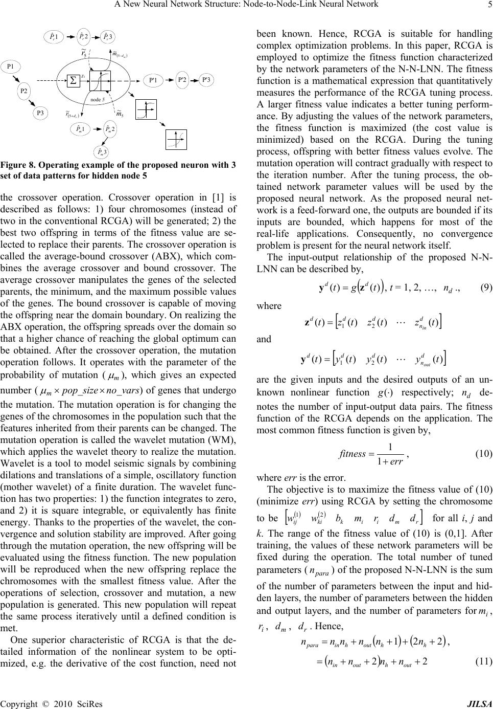

A New Neural Network Structure: Node-to-Node-Link Neural Network5
P1
P2

5
~
r

r
d
r
5
~

m
d
m
5
~
5
~
m
5

P'1
node 5
P3
P'2 P'3
1
ˆ
r
P
2
ˆ
r
P 3
ˆ
r
P
1
ˆ
m
P2
ˆ
m
P
3
ˆ
m
P
Figure 8. Operating example of the proposed neuron with 3
set of data patterns for hidden node 5
the crossover operation. Crossover operation in [1] is
described as follows: 1) four chromosomes (instead of
two in the conventional RCGA) will be generated; 2) the
best two offspring in terms of the fitness value are se-
lected to replace their parents. The crossover operation is
called the average-bound crossover (ABX), which com-
bines the average crossover and bound crossover. The
average crossover manipulates the genes of the selected
parents, the minimum, and the maximum possible values
of the genes. The bound crossover is capable of moving
the offspring near the domain boundary. On realizing the
ABX operation, the offspring spreads over the domain so
that a higher chance of reaching the global optimum can
be obtained. After the crossover operation, the mutation
operation follows. It operates with the parameter of the
probability of mutation (m

), which gives an expected
number ( pop_size
m

no_vars) of genes that undergo
the mutation. The mutation operation is for changing the
genes of the chromosomes in the population such that the
features inherited from their parents can be changed. The
mutation operation is called the wavelet mutation (WM),
which applies the wavelet theory to realize the mutation.
Wavelet is a tool to model seismic signals by combining
dilations and translations of a simple, oscillatory function
(mother wavelet) of a finite duration. The wavelet func-
tion has two properties: 1) the function integrates to zero,
and 2) it is square integrable, or equivalently has finite
energy. Thanks to the properties of the wavelet, the con-
vergence and solution stability are improved. After going
through the mutation operation, the new offspring will be
evaluated using the fitness function. The new population
will be reproduced when the new offspring replace the
chromosomes with the smallest fitness value. After the
operations of selection, crossover and mutation, a new
population is generated. This new population will repeat
the same process iteratively until a defined condition is
met.
One superior characteristic of RCGA is that the de-
tailed information of the nonlinear system to be opti-
mized, e.g. the derivative of the cost function, need not
been known. Hence, RCGA is suitable for handling
complex optimization problems. In this paper, RCGA is
employed to optimize the fitness function characterized
by the network parameters of the N-N-LNN. The fitness
function is a mathematical expression that quantitatively
measures the performance of the RCGA tuning process.
A larger fitness value indicates a better tuning perform-
ance. By adjusting the values of the network parameters,
the fitness function is maximized (the cost value is
minimized) based on the RCGA. During the tuning
process, offspring with better fitness values evolve. The
mutation operation will contract gradually with respect to
the iteration number. After the tuning process, the ob-
tained network parameter values will be used by the
proposed neural network. As the proposed neural net-
work is a feed-forward one, the outputs are bounded if its
inputs are bounded, which happens for most of the
real-life applications. Consequently, no convergence
problem is present for the neural network itself.
The input-output relationship of the proposed N-N-
LNN can be described by,

 )()( tgt dd zy , t = 1, 2, …, ., (9)
d
n
where

 )()()()( 21 tztztzt d
n
ddd
in
z
and

 )()()()( 21tytytyt d
n
ddd
out
y
are the given inputs and the desired outputs of an un-
known nonlinear function respectively; de-
notes the number of input-output data pairs. The fitness
function of the RCGA depends on the application. The
most common fitness function is given by,
)(gd n
err
fitness  1
1, (10)
where err is the error.
The objective is to maximize the fitness value of (10)
(minimize err) using RCGA by setting the chromosome
to be
 


rmiikkiij ddrmbww 21
para
n
m r
d
for all i, j and
k. The range of the fitness value of (10) is (0,1]. After
training, the values of these network parameters will be
fixed during the operation. The total number of tuned
parameters () of the proposed N-N-LNN is the sum
of the number of parameters between the input and hid-
den layers, the number of parameters between the hidden
and output layers, and the number of parameters for,
, , . Hence,
i
m
i
r d
 221  


hhouthinpara nnnnnn ,


22



outhoutin nnnn (11)

A New Neural Network Structure: Node-to-Node-Link Neural Network 6
4. Industrial Application and Results
In this section, industrial application example will be
given to illustrate the merits of the proposed network.
The application is on hand-written graffiti recognition.
A hand-written graffiti pattern recognition problem is
used to illustrate the superior learning and generalization
abilities of the proposed network on a classification
problem with a large number of input data sets. In gen-
eral, the neural network approaches are model-free. Dif-
ferent kinds of neural model applied for hand-written
recognition system are reported in [8,10,12,15,16].
4.1 Neural Network Based Hand-Written
Graffiti Recognition System
In this example, the digits 0 to 9 and three control cha-
racters (backspace, carriage return and space) are rec-
ognized by the N-N-LNN. These graffiti are shown in
Figure 9. A point in each graffiti is characterized by a
number based on the x-y coordinates on a writing area.
The size of the writing area is xmax by ymax. The bottom
left corner is set as (0, 0). Ten uniformly sampled points
of the graffiti will be taken in the following way. First,
the input graffiti is divided into 9 uniformly distanced
segments characterized by 10 points, including the start
and the end points. Each point is labeled as (xi, yi), i = 1,
2, …, 10. The first 5 points, (xi, yi), i = 1, 3, 5, 7 and 9
taken alternatively are converted to 5 numbers zi respec-
tively by using the formula zi = xixmax+ y
i. The other 5
points, (xi, yi), i = 2, 4, 6, 8 and 10 are converted to 5
numbers respectively by using the formula zi = yiymax+ xi.
These ten numbers, zi, i = 1, 2, …, 10, are used as the
inputs of the proposed graffiti recognizer. The
hand-written graffiti recognizer as shown in Figure 10 is
proposed. Its inputs are defined as follows,
)(
)(
)( t
t
tz
z
z, (12)
where

)()()()( 1021tztztzt z
Digits/
Chars Strokes Digits/ Chars Strokes Digits/ Chas Strokes
0(a)
5(a) 9
0(b)
5(b) Back-space
1
6
Carriage
Return
2 7
Space
3 8(a)
4
8(b)
Figure 9. Graffiti digits and characters (with the dot indi-
cating the starting point of the graffiti)
Neural
Network
with
Adaptive
Activation
Functions
)(
1tz
)(
2tz
)(
10 tz
)(
1
t
y
)(
2ty
)(
16 ty
Graffiti
Determiner Output


NNAAF
Figure 10. Graffiti digits and characters (with the dot indi-
cating the starting point of the graffiti)

denotes the
normalized input vectors of the proposed graffiti recog-
nizer; denotes the ten
points in the writing area;
 )()()()( 1021 tztztzt z
 denotes the l2 vector norm.
The 16 outputs, , k = 1, 2, …, 16, indicates the
similarity between the input pattern and the 16 standard
patterns respectively. The input-output relationship of the
training patterns is defined such that the output
)(tyk
1)(

tyi
and others are zero when the input vector belongs to pat-
tern i, i = 1, 2, …, 16. For example, the desired outputs of
the pattern recognition system are [1 0 0 0 0 0 0 0 0 0 0 0
0 0 0 0] for the digit “0(a)”, [0 1 0 0 0 0 0 0 0 0 0 0 0 0 0
0] for the digit “0(b)”, and [0 0 0 0 0 0 0 0 0 0 0 0 0 0 0 1]
for the character “space” respectively. After training, a
graffiti determiner is used to determine the output of the
graffiti. A larger value of implies that the input
pattern matches more closely to the corresponding graf-
fiti pattern. For instance, a large value of implies
that the input pattern is recognized as “0”.
)(ty j
)(
0ty
4.2 Results and Analysis
To train the neural network of the hand-written graffiti
recognition system, a set of training pattern governing
the input-output relationship will be used. 1600 training
patterns (100 patterns for each graffiti) will be used in
this example. The training patterns consist of the input
vectors and its corresponding expected output. The fit-
ness function is given by (10), with













16
1
100
1
2
10016
)(
)(
)(
)(
k
td
d
kk
t
ty
t
ty
err
y
y
,
(13)

A New Neural Network Structure: Node-to-Node-Link Neural Network 7

where

)()()()( 1621tytytyt ddddy
Table 1. Training results on doing the hand-written graffiti
recognition
denotes the expected output vector and
 )()()()( 1621 tytytyt y
18
h
n 20
h
n 22
h
n24

h
n
para
n 520 576 632 688
MSE 0.01850.0157 0.0169 0.0179Ave.
training Acc. 96.50% 97.38% 96.85% 96.62%
MSE 0.01680.0139 0.0145 0.0143
N-N-LNN
Best
trainingAcc.96.88% 98.06% 97.31% 97.38%
para
n 1004 1112 1220 1328
MSE0.03370.0328 0.0314 0.0322Ave.
training Acc. 92.46% 92.62% 93.25% 93.18%
MSE0.03090.0293 0.0282 0.0288
FSNLS
Best
training Acc. 93.40% 93.75% 94.00% 93.86%
para
n 486 540 594 648
MSE0.03490.0321 0.03160.0309 Ave.
training Acc. 92.35% 92.42% 93.10%93.23%
MSE0.03150.0292 0.02800.0278
WNN
Best
training Acc. 93.31% 93.81% 94.00%94.13%
para
n 502 556 610 664
MSE0.03930.0385 0.03800.0360 Ave.
trainingAcc.90.17% 90.46% 90.73%91.50%
MSE0.03700.0388 0.03610.0326
FFCNN
Best
trainingAcc.90.50% 91.69% 92.56%93.06%
is the actual network output defined as,





 

h
i
n
ikskik btfwtfty 1
)2(
2))(()( z, k = 1, 2, …, 16, (14)
where
 







trtmtzwtftzf ii jjijsi
~
,
~
,)())(( 10
1
)1(
1, i = 1, 2, …,nh, (15)
where tf2() is a pure linear transfer function in this app-
lication.
For comparison purposes, a conventional 3-layer fully
connected feed-forward neural network (FFCNN) [11], a
fixed-structure network with link switches (FSNLS) [6],
and a wavelet neural network (WNN) [14, 17–18 ] (which
combines feed-forward neural networks with the wavelet
theory, providing a multi-resolution approximation for
discriminate functions) trained by the improved RCGA
[1] are also used in this example. For all cases, the initial
values of the parameters of the neural network are ran-
domly generated. In this application, the lower and upper
bounds of the network parameters of the N-N- LNN
are , and
. For the FSNLS, WNN and
FFCNN, the network parameters are ranged from –4 to 4.
The number of iterations to train the neural networks is
15000. For the RCGA [1], the probability of crossover
(

 44
)2()1( 
ikkiij mbww
   11  hrm nd
c

25.0
i
r
d

) and the probability of mutation (m

) are 0.8 and
0.05 respectively; the weights of the average-bound
crossover and are set at 0.5 and 1 respectively;
the shape parameter of wavelet mutation
a
wb w

is 2, and
the population size is 50. All the results are the averaged
ones out of 20 runs. In order to test the generalization
ability of the proposed neural networks, a set of testing
patterns consisting of 480 input patterns (30 patterns for
each graffiti) is used.
Table 2. Training results on doing the hand-written graffiti
recognition
18
h
n 20
h
n 22
h
n24

h
n
para
n 520 576 632 688
MSE520 576 632 688 Ave.
trainingAcc. 0.02280.0186 0.0199 0.0211
MSE95.21% 96.96% 95.49% 95.40%
N-N-LNN
Best
training Acc.0.02040.0171 0.01850.192
para
n 95.93%
97.29% 96.25% 96.05%
MSE1004 1112 1220 1328 Ave.
trainingAcc. 0.03630.0350 0.0331 0.0349
MSE92.28% 92.50% 93.21%93.00%
FSNLS
Best
trainingAcc. 0.03300.0322 0.0310 0.0312
para
n 92.92% 93.13%
93.96%93.75%
MSE486 540 594 648 Ave.
trainingAcc. 0.03650.0346 0.03440.0329
MSE92.08% 92.22% 92.71%93.92%
WNN
Best
trainingAcc. 0.03290.0320 0.03220.0308
para
n 92.59% 93.54% 93.75%94.38%
MSE502 556 610 664 Ave.
trainingAcc.0.04100.0404 0.03930.0374
MSE90.07% 90.58% 90.68%91.25%
FFCNN
Best
trainingAcc.0.04040.0393 0.03880.0361
The average training, best training, average testing and
best testing results in terms of mean square error (MSE),
and the recognition accuracy rate of all approaches are
summarized in Table 1 and Table 2. It can be seen from
these two tables that the recognition system implemented
by the N-N-LNN outperforms those by the FSNLS,
WNN and FFCNN. The best results are achieved when
the number of hidden nodes (nh) is set at 20 for the
N-N-LNN, nh = 22 for the FSNLS, and nh = 24 for the
WNN and FFCNN. In comparison with the FSNLS,
WNN and FFCNN, the average training and testing er-
rors of N-N-LNN at nh = 20 are 0.0157 and 0.0186 re-
spectively. They imply 77.96% improvement over
FSNLS at nh = 22, 96.82% and 76.90% improvement
over WNN at nh = 24, and 129.3% and 101.1% im-
provement over FFCNN at nh = 24, respectively. In terms
of the average testing recognition accuracy rate, the
N-N-LNN (96.96%) gives a better result than the FSNLS
(93.21%), WNN (93.92%) and FFCNN (91.25%).
Figure 11 shows the selected output values of the

A New Neural Network Structure: Node-to-Node-Link Neural Network 8
N-N-LNN
030 6090 120 150 180 210240 270300 330 360 390 420450 480
-0.5
0
0.5
1
pattern number
output y
030 6090120 150 180 210 240 270 300 330 360390 420 450480
-0.5
0
0.5
1
pattern number
output y
FSNLS
030 60 90 120 150 180 210 240 270 300 330360 390 420450 480
-0. 5
0
0. 5
1
pattern number
output y
030 60 90120 150180 210 240 270 300330 360390 420 450480
-0. 5
0
0.5
1
pattern number
output y
WNN
030 6090 120 150 180210240 270300 330360 390 420450 480
-0.5
0
0.5
1
pattern number
output y
030 6090120 150 180 210 240 270 300 330 360390 420 450480
-0.5
0
0.5
1
pattern number
output y
FFCNN
030 6090 120 150 180210240 270 300 330360 390 420450 480
-0.5
0
0.5
1
pattern number
output y
030 60 90120150180 210240 270 300330 360390 420 450480
-0.5
0
0.5
1
pattern number
output y
(a). Digit ‘0’(b). (b). Digit ‘6’.
Figure 11. Output values of the N-N-LNN, FSNLS, WNN, and FFCNN for the 480 (30 for each type) testing graffiti patterns

A New Neural Network Structure: Node-to-Node-Link Neural Network 9
N-N-LNN
030 6090120 150180 210240 270 300330 360390 420 450480
-0.5
0
0.5
1
pattern number
output y
030 6090120 150180 210240 270 300330 360390 420 450480
-0.5
0
0.5
1
pattern number
output y
FSNLS
030 60 90120 150 180 210240 270 300330 360390 420 450480
-0.5
0
0.5
1
pattern number
output y
030 6090120 150180 210240 270 300330 360390 420 450480
-0.5
0
0.5
1
pattern number
output y
WNN
030 60 90120 150 180 210240 270 300330 360390 420 450480
-0.5
0
0.5
1
pattern number
output y
030 6090120 150180 210240 270 300330 360390 420 450480
-0.5
0
0.5
1
pattern number
output y
FFCNN
030 6090120 150 180 210 240 270 300 330 360390 420 450480
-0.5
0
0.5
1
pattern number
output y
030 6090120 150180 210240 270 300330 360390 420 450480
-0.5
0
0.5
1
pattern number
output y
(c). Digit ‘carriage return’. (d). Digit ‘space’..
Figure 11 (continued). Output values of the N-N-LNN, FSNLS, WNN, and FFCNN for the 480 (30 for each type) testing graf-
fiti patterns

A New Neural Network Structure: Node-to-Node-Link Neural Network 10
N-N-LNN, FSNLS, WNN and FFCNN for the 480 (30
for each digit/character) testing graffiti. In this figure, the
x-axis represents the pattern number for corresponding
digit/character. The pattern numbers 1 to 30 are for the
digit “0(a)”, the numbers 31-60 are for the digit “0(b)”,
and so on. The y-axis represents the output yi. As men-
tioned before, the input-output relationship of the pat-
terns will drive the output and other outputs
are zero when the input vector belongs to pattern i, i = 1,
2, …, 16. For instance, the desired output y of the pattern
recognition system is [0 1 0 0 0 0 0 0 0 0 0 0 0 0 0 0] for
1)( tyi
digit “0(b)”. Referring to Figure 11(d), we can see that
the output y16 of the N-N-LNN for pattern numbers
within 451-480 (the character “space”) is nearest to 1 and
other outputs are nearest to zero. It shows that the recog-
nition accuracy rate achieved by the N-N-LNN is good.
5. Conclusions
A new neural network has been proposed in this paper.
The parameters of the proposed neural network are
trained by the RCGA. In this topology, the parameters of
the activation function in the hidden nodes are changed
according to the input to the network and the outputs of
other hidden-layer nodes in the network. Thanks to the
variable property and the node-to-node links in the hid-
den layer, the learning and generalization abilities of the
proposed network have been increased. Application on
hand-written graffiti recognition has been given to illus-
trate the merits of the proposed N-N-LNN. The proposed
network is effectively an adaptive network. By adaptive,
we mean the network parameters are variable and depend
on the input data. For example, when the proposed neu-
rons of the N-N-LNN manipulate an input pattern, the
shapes of the activation functions are characterized by
the inputs from the upper and lower neighbour’s outputs,
which depend on the input pattern itself. In other words,
the activation functions, or the parameters of the N-N-
LNN, are adaptively varying with respect to the input
patterns to produce the outputs. All network parameters
of the N-N-LNN depend only on the present state. That
means the network is a feed-forward one, causing no
stability problem to the network dynamics.
REFERENCES
[1] S. H. Ling and F. H. F Leung, “An improved genetic
algorithm with average-bound crossover and wavelet
mutation operations,” Soft Computing, Vol. 11, No.1, pp.
7–31, January 2007.
[2] F. M. Ham and I. Kostanic, “Principles of neurocomput-
ing for science & engineering,” McGraw Hill, 2001.
[3] R. C. Bansal and J. C. Pandey, “Load forecasting using
artificial intelligence techniques: A literature survey,” In-
ternational Journal of Computer Applications in Tech-
nology, Vol. 22, Nos. 2/3, pp. 109–119, 2005.
[4] S. H. Ling, F. H. F. Leung, H. K. Lam, and P. K. S. Tam,
“Short-term electric load forecasting based on a neural
fuzzy network,” IEEE Transactions on Industrial Elec-
tronics, Vol. 50, No. 6, pp. 1305–1316, December 2003.
[5] S. H. Ling, F. H. F. Leung, L. K. Wong, and H. K. Lam,
“Computational intelligence techniques for home electric
load forecasting and balancing,” International Journal
Computational Intelligence and Applications, Vol. 5, No.
3, pp. 371–391, 2005.
[6] F. H. F. Leung, H. K. Lam, S. H. Ling, and P. K. S. Tam,
“Tuning of the structure and parameters of neural network
using an improved genetic algorithm,” IEEE Transactions
on Neural Networks, Vol. 14, No. 1, pp. 79–88, January
2003.
[7] K. F. Leung, F. H. F. Leung, H. K. Lam, and S. H. Ling,
“On interpretation of graffiti digits and commands for
eBooks: Neural-fuzzy network and genetic algorithm app-
roach,” IEEE Transactions on Industrial Electronics, Vol.
51, No. 2, pp. 464–471, April 2004.
[8] D. R. Lovell, T. Downs, and A. C. Tsoi, “An evaluation
of the neocognitron,” IEEE Transactions on Neural Net-
works, Vol. 8, No. 5, pp. 1090–1105, September 1997.
[9] Z. Michalewicz, “Genetic algorithm + data structures =
evolution programs,” 2nd extended edition, Springer-Ver-
lag, 1994.
[10] C. A. Perez, C. A. Salinas, P.A. Estévez, and P. M.
Valenzuela, “Genetic design of biologically inspired re-
ceptive fields for neural pattern recognition,” IEEE
Transactions on Systems, Man, and Cybernetics — Part B:
Cybernetics, Vol. 33, No. 2, pp. 258–270, April 2003.
[11] B. Widrow and M. A. Lehr, “30 years of adaptive neural
networks: Perceptron, madaline, and backpropagation,”
Proceedings of the IEEE, Vol. 78, No. 9, pp. 1415–1442,
September 1990.
[12] R. Buse, Z. Q. Liu, and J. Bezdek, “Word recognition
using fuzzy logic,” IEEE Transactions on Fuzzy Systems,
Vol. 10, No. 1, February 2002.
[13] L. Davis, “Handbook of genetic algorithms,” NY: Van
Nostrand Reinhold, 1991.
[14] X. Yao, “Evolving artificial networks,” Proceedings of
the IEEE, Vol. 87, No. 7, pp. 1423–1447, 1999.
[15] P. D. Gader and M. A. Khabou, “Automatic feature gen-
eration for handwritten digit recognition,” IEEE Transac-
tions on Pattern Analysis and Machine Intelligence, Vol.
18, No. 12, pp. 1256–1261, December 1996.
[16] L. Holmström, P. Koistinen, J. Laaksonen, and E. Oja,
“Neural and statistical classifiers — Taxonomy and two
case studies,” IEEE Transactions on Neural Networks,
Vol. 8, No. 1, pp. 5–17, January 1997.
[17] J. Zhang, G. G. Walter, Y. Miao, and W. W. N. Lee,
“Wavelet neural networks for function learning,” IEEE
Transactions on Signal Processing, Vol. 43, No. 6, pp.
1485–1497, June 1995.
[18] B. Zhang, M. Fu, H. Yan, and M. A. Jabri, “Handwritten
digit recognition by adaptive-subspace self-organizing
map (ASSOM),” IEEE Transactions on Neural Networks,

A New Neural Network Structure: Node-to-Node-Link Neural Network 11
Vol. 10, No. 4, pp. 939–945, July 1997.
[19] C. K. Ho and M. Sasaki, “Brain-wave bio potentials
based mobile robot control: Wavelet-neural network pat-
tern recognition approach,” in Proceedings IEEE Interna-
tional Conference on System, Man, and Cybernetics, Vol.
1, pp. 322–328, October 2001.
[20] S. Yao, C. J. Wei, and Z. Y. He, “Evolving wavelet neu-
ral networks for function approximation,” Electron Letter,
Vol.32, No.4, pp. 360–361, February 1996.
[21] Q. Zhang and A. Benveniste, “Wavelet networks,” IEEE
Transactions on Neural Networks, Vol. 3, No. 6, pp.
889–898, November 1992.