Int'l J. of Communications, Network and System Sciences
Vol.2 No.5(2009), Article ID:606,11 pages DOI:10.4236/ijcns.2009.25047
Load Control for Overloaded MPLS/DiffServ Networks during SLA Negotiation
1University of Dubrovnik, Department of Electrical Engineering and Computing, Dubrovnik, Croatia
2University of Zagreb, Faculty of Transport and Traffic Engineering, Zagreb, Croatia
Email: srecko.krile@unidu.hr, dragan.perakovic@fpz.hr
Received April 16, 2009; revised May 20, 2009; accepted July 2, 2009
Keywords: End-To-End Qos Provisioning, Traffic Engineering In MPLS/Diffserv Networks,Constraint-Based Routing, Load Control during SLA Creation
ABSTRACT
In end-to-end QoS provisioning some bandwidth portions on the link may be reserved for certain traffic classes (and for particular set of users) so the congestion problem of concurrent flows (traversing the network simultaneously) can appear. It means that in overloaded and poorly connected MPLS/DS networks the CR (Constraint-based Routing) becomes insufficient technique. If traffic engineering is supported with appropriate traffic load control the congestion possibility can be predicted before the utilization of guaranteed service. In that sense the initial (pro-active) routing can be pre-computed much earlier, possible during SLA (Service Level Agreement) negotiation. In the paper a load simulation technique for load balancing control purpose is proposed. It could be a very good solution for congestion avoidance and for better load-balancing purpose where links are running close to capacity. To be acceptable for real application such complicated load control technique needs very effective algorithm. Proposed algorithm was tested on the network with maximum M core routers on the path and detail results are given for N=3 service classes. Further improvement through heuristic approach is made and results are discussed. Some heuristic options show significant complexity savings that is appropriate for load control in huge networks.
1. Introduction
The core network for NGN (New Generation Network) is evolving to MPLS/DiffServ based network. With capability in service differentiation techniques the network operator can ensure the traffic priorization, specialy to quality voice (VoIP) and video calls (premium traffic), as same as for truly differentiated data services. It means that DiffServ classifies individual flows in a small number of service classes (at network edges). Also it enables ‘’soft’’ reservation (allocation) of resources and special handling of packets in the core. Together, MPLS (Multi Protokol Label Switching) and DiffServ provide a scalable QoS solution for the core of NGN; see [1] and [2].
MPLS uses extensions to Resource Reservation Protocol (TE-RSVP) and the MPLS forwarding paradigm to provide explicit routing; see [3-5]. But end-to-end provisioning of coexisted and aggregated traffic in networks is still demanding problem, specially if overprovisioning is not possible. All traffic flows in domain are distributed among LSPs (Label Switching Path) related to N service classes, but we know the IGP (Interior Getaway Protocol) uses simple on-line routing protocols (e.g. OSPF, IS-IS) based on shortest path methodology. With OSPF (Open Shortest Path First) some paths may become congested while others are underutilized. Constraint-based routing (CR) as an extension of explicit routing ensures traffic engineering (TE) capabilities. CSPF (Constrained Shortest Path First) allows an originating (ingress) router to compute a path (LSP) to egress router (sequence of intermediate LSRs), taking care of constraints such as bandwidth, delay and administrative policy; see [12]. It can find out a longer but lightly loaded path, better than the heavily loaded shortest path. With constraint-based label distribution protocol (CR-LDP) the bandwidth provisioning directives and other information can be ensured (list of router's neighbors, attached networks, actual resource availability and other relevant information). It can be distributed for each service class and for each link along the path (LSP); see [6]. CR process can be incorporated into each ingress router and co-exists with the conventional routing technique.
MPLS/DiffServ aware TE (DS-TE) allows constraintbased routing of IP traffic with final task to adjust class load to actual class capacity. But the routing approach explained above can be effective in under loaded networks or in fully connected networks only. For them the RED or WRED (Weighted Random Early Detection) are effective congestion avoidance techniques. But in some networks dropping packets can lead to customer dissatisfaction and SLA violation. In the context of simultaneous flows (former contracted SLAs + new SLA creation) bandwidth overbooking is possible and congestion problem during service utilization can appear. For overloaded and poorly connected networks we need prediction of congestion probability much earlier. Load balancing has to be done much before the moment of service utilization, possibly during SLA negotiation process. To obtain quantitative end-to-end guarantees the QoS provisioning has to be in firm correlation with bandwidth management; see [7,8]. Also, such load control as a part of DS-TE can help in optimal bandwidth reservation, to predict sufficient resources and to ensure better end-to-end QoS provisioning, see [14]. TE involves the management of existing bandwidth resources to suit trafic demands and to meet the growing demands of customers in the network.
New approach in load control during SLA creation is given in Section 2. Load control can be seen as the capacity expansion problem (CEP) of N capacity types. Expansions are possible in given limits for each bandwidth portion (sub-pool), influencing on each other. The mathematical model explanation for CEP is given in the Section 3. In the Section 4, we have CEP algorithm development and heuristic approach. The comparison of results for different algorithm options we can see in the Section 5.
2. LSP Creation during SLA Negotiation
The service provider for domain (e.g. ISP) wants to accept a new SLA that results with priority traffic flow between edge routers. A traffic trunk is defined as a logical pipeline within an LSP, with reservation of certain amount of capacity to serve the traffic associated with a certain SLA. So it is clear that LSP between an ingress/egress pair may carry multiple traffic trunks associated with different SLAs; see [10]. In Figure 2 we have situation on the path for the example of simultaneous SLA flows from Figure 1. All traffic flows on the path are participating possibly in the same time (the worst case). In that sense the network operator (e.g ISP) has to find the optimal LSPs for aggregated flows without any possible congestion in the core network; see [9]. Each traffic demand can be satisfied on appropriate or higher QoS level, using appropriate bandwidth portion from a sub-pool. The main condition is: the sufficient network resources must be available for the priority traffic at any moment.
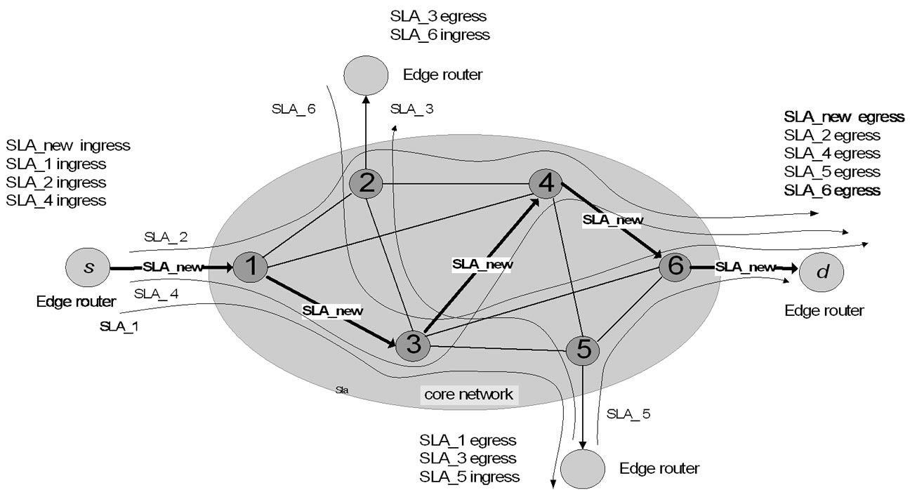
Figure 1. An example of number of flows (former SLAs) in the context of new SLA creation.
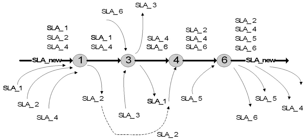
Figure 2. Simultaneous flows with possibly congestion on the path.
So we propose the next scenario: during SLA negotiation process the RM (Resource Manager) module has to determine the main parameters that characterize the required flow (i.e., bandwidth, QoS class, ingress and egress IP router addresses, time of service utilization); see [13]. At first RM can apply off-line routing to get initial LSP, taking care of all other simultaneous flows. It can be done with any shortest path-based routing algorithm (e.g. OSPF). From RM we can get statistical details for each SLA flow traversing the network simultaneously, e.g. ingress node, egress node, service class, bandwidth etc.). We need very effective algorithm to simulate such traffic load and detect congestion possibility on the path. Such optimization is a multi-constrained problem (MCP).
The BB (Bandwidth Broker) will check if there are enough resources on the calculated path to satisfy the requested service class. If such calculated path has any link that exceeds allowed capacity limits (maximal bandwidth for appropriate service class) possible congestion exists; see [15]. It means that link capacity on the path cannot be sufficient for new traffic load. Alternatively, adding capacity arrangement (dynamic bandwidth reservation) for congested link has to be done but it may produce significant extra cost. Abut dynamic bandwidth reservation mechanism we can see in [20] and [21].
If calculation finds that proposed path has no any congestion the new SLA can be accepted and related LSP is assigned to that traffic flow (SLA) and stored in database of RM. In opposite the new SLA cannot be accepted or must be re-negotiated. In the moment of service invocation such calculated (and stored) LSP can be easily distributed from RM to the MPLS network to support explicit routing, leveraging bandwidth reservation and prioritization; see [16].
In that way the LSP creation should be in co-relation with SLA, to enable better load-balancing and to ensure congestion avoidance in domain. Also, such load balancing technique is appropriate for inter-domain end-to-end path provisioning in the part of optimal bandwidth reservation from neighbor ASes (Autonomous System). Capacity reservations have to be done in the most effective way in order to provide bandwidth guarantees for predicted traffic; see [11]. Having purchased access to sufficient bandwidth from downstream ASes, home AS can utilize both: purchased bandwidth and its own network capacity.
3. Mathematic Model of CEP for Congestion Control and Load Balancing Purpose
The congestion control technique explained above can be seen as the capacity expansion problem (CEP) on the path with or without shortages. If the fulfillment of traffic demand is the main condition we talk about CEP without shortages. Transmission link on the path are capable to serve traffic demands for N different QoS levels (service class) for i = 1, 2, ..., N. For each traffic load we need appropriate bandwidth amount, so it looks like bandwidth expansion. Bandwidth portions on the link can be assigned to traffic flow of appropriate service class up to the given limit of bandwidth sub-pool (maximal capacity for defined service class). Used capacity can be increased in two forms: by expansion or by conversion. Expansions can be done separately for each service class or through conversion (redirected amount) to lower quality class. It means that capacity can be reused to serve the traffic of lover quality level under special conditions. For example, if capacity predefined for priority traffic is unused it can be redirected to support best effort services. Bandwidth usage for each service class (sub-pool) can be a part of resource reservation strategy but sum of all sub-pools has to be equal/less than link capacity. Figure 3 gives an example of network flow representation for network flow for multiple QoS levels (N) and M core routers (LSR) and M+1 links on the path.

Figure 3. The network flow representation of the CEP for Russian Dolls bandwidth allocation model.
Network has V core routers, M £ V, and A links connecting all of them, including edge routers.
In the CEP model the following notation is used:
i, j and k = QoS level. We differentiate n service classes (QoS levels).The N levels are ranked from i = 1, 2,..., N, from higher to lower.
m = on the path, connecting two successive routers m1 and m2, m = 1, …., M+1.
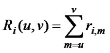
ri,m = traffic demand increment for additional capacity on the link m from appropriate sub-pool i. For convenience, the ri.m is assumed to be integer. For the flow going out from the path ri,m is negative. The sum of traffic demands for capacity type i between two routers on the path:
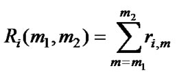 (1)
(1)
xi,m = the amount of adding capacity for appropriate service class i on the link m. Possible negative values – decrease. It means that we have idle (sufficient) capacity. If dynamic bandwidth management is possible such reduction can be realized.
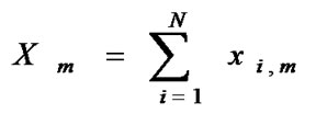 (2)
(2)
The sum of demands for whole path and for all capacity types has to be positive or zero (including new SLA):
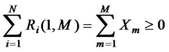 (3)
(3)
From this formulation it is obvious that sum of traffic demands on the path has to be equal to capacity amount used to satisfy them. It means that we don’t expect reduction of total capacity on the path toward egress router, in other words we presume the increase of capacity.
yi,j,m = the amount of capacity for quality level i on the link m, redirected to satisfy the traffic of lower quality level j.
Any traffic demand can also be satisfied by converted capacity from any capacity type k < i with higher quality level. In Figure 3, such flows are marked with doted lines.
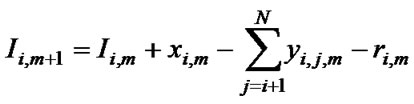
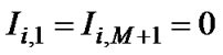
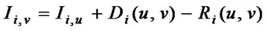
Ii,m = relative amount for the capacity type i on the link m, connecting two neighbor routers. Idle capacity is represented with positive value. If shortages are not allowed negative value cannot exist. Ii1 = 0, Ii,M+1 = 0 that means: no adding capacity is necessary on the link toward edge routers. It means that the capacity for that link is always sufficient.
Li,m = bandwidth constraints for link capacity values on the link m and for appropriate service class i (L1,m , L2,m , … LN,m).
wi,m= weight for the link m and appropriate service class i (QoS level).
deli,m= delay on the link m for appropriate service class i. Maximal delay on the path is denoted with DELi .
As we have nonlinear expansion functions (showing the economy of scale) the CEP can be solved by any nonlinear optimization technique. Instead of polynomial optimization (e.g. nonlinear convex programming), that can be very complicated (NP-complete), the network optimization methodology is efficiently applied. The main reason on such approach is the possibility of discrete capacity values for limited number of QoS classes, so the optimization can be significantly improved. The problem can be formulated as Minimum Cost Multi-Commodity Flow Problem (MCMCF). Such problem can be easily represented by multi-commodity the single (common) source multiple destination network; see Figure 3.
Let G (V, A) denote a network topology, where V is the set of vertices(nodes), representing link capacity states and A, the set of arcs, representing traffic flows between routers. Each link on the path is characterized by z-dimensional link weight vector, consisting of z-nonnegative QoS weights. The number of QoS measures (e.g. bandwidth, delay) is denoted by z. In general we have multi-constrained problem (MCP) but in this paper we talk about one-dimensional link weight vectors for M+1 links on the path {wi,m, m Î A, i = 1, …, N}. E.g. the capacity constraint for each link on the path is denoted with Li,m (L1,m L2,m, … LN,m). For non-additive measures (e.g. for bandwidth where the cost-function is concave, and we are looking for minimum) definition of the singleconstrained problem is to find a path from ingress to egress node with minimal link weight along the path.
In the context of MCP we can introduce easily the adding constraint of max. Delay on the path (end-to-end). As it is an additive measure (more links on the path cause higher delay) it can be used as criteria to eliminate any unacceptable capacity expansion solution from calculation.
The flow situation on the link depends of expansion and conversion values (xi,m , yi,j,m). It means that the link weight (cost) is the function of used capacity: lower amount of used capacity (capacity utilization) gives lower weight. If the link expansion cost corresponds to the amount of used capacity, the objective is to find the optimal expansion policy that minimizes the total cost on the path. Definition of the single-constrained problem is to find a path P from ingress to egress node such that:
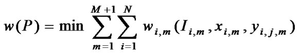 (4)
(4)
where:
Ii,m £ Li,m (5)
satisfying condition of max. Delay for P:
 (6)
(6)
for i = 1, …, N ; m = 1,…, M A path obeying the above conditions is said to be feasible. Note that there may be multiple feasible paths between ingress and egress node. Generalizing the concept of the capacity states for each quality level of transmission link m between LSRs in which the capacity states for each service class (QoS level) are known within defined limits we define a capacity point - am.
am = (I1,m, I2,m, ... , IN,m) (7)
a1 = aM+1 = (0, 0, ... , 0) (8)
In formulation (3.7) am denotes the vector of capacities Ii,m for each service class on link m, and we call it capacity point. On the flow diagrams (Figure 2) each column represents a capacity point of the node, consisting of N capacity state values (for i-th QoS level). Link capacity is capable to serve different service classes. Capacity amount labeled with i is primarily used to serve traffic demands of that service class but it can be used to satisfy traffic of lower QoS Level j (j > i).
Formulation (3.8) implies that idle capacities or capacity shortages are not allowed on the beginning and on the end of the path. It means that process is starting with new SLA flow that must be fully satisfied through the network (from ingress to egress node).
The objective function for CEP problem can be formulated as follows:
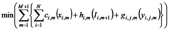 (9)
(9)
so that we have:
 (10)
(10)
 (11)
(11)
for m = 1, 2, ..., M+1; i = 1, 2, ... , N; j = i + 1, ... , N.
In the objective function (3.9) the total cost (weight) includes some different costs. Expansion cost (adding capacity) is denoted with ci,m (xi,m). For the link expansion in allowed limits we can set the expansion cost to zero. We can differentiate expansion cost for each service class. We can take in account the idle capacity cost hi,m (Ii,m+1), but only as a penalty cost to force the usage of the minimum link capacity (prevention of unused/idle capacity). Also we can introduce facility conversion cost gi,j,m (yi,j,m) that can control non‑effective usage of link capacity (e.g. usage of higher service class capacity instead). Costs are often represented by the fix-charge cost or with constant value. We assume that all cost functions are concave and non-decreasing (reflecting economies of scale) and they differ from link to link. The objective function is necessarily non-linear cost. With different cost parameters we can influence on the optimization process, looking for benefits of the most appropriate expansion solution.
4. Algorithm Development
The network optimization can be divided in two steps. At first step we are calculating the minimal expansion weight du,v for capacity expansion between two capacity points of neighbor links. It has to be done for all capacity points and for all pairs of neighbor routers (interconnected).
u,v = the order number of capacity points in the sub-problem for appropriate link, 1 £ u, ..., v £ M+1.
The calculation of weight value between two capacity points we call: capacity expansion sub-problem (CES); see (4.1). The expansion sub-problem for N facilities i = 1, 2, … , N on the path between routers u and v is as:
 (12)
(12)
where:
 (13)
(13)
 (14)
(14)
Di (u,v)=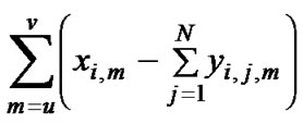 ; i¹ j (15)
for m = 1, 2, ... , M+1; i = 1, 2, ... , N; j = i + 1, ... , N.
Let Cm be the number of the capacity point values for link m between two neighbor core routers. Only one capacity point for the link that connects the edge router: C1 = CM+1 = 1.
The total number of capacity points is:
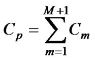 (16)
(16)
In the CEP we have to find many cost values du,v(au, av) that emanate two capacity points, from each node (u, au) to node (v, av) for v ³ u. The total number of CES can be pretty large:
 (17)
(17)
For every CES the calculation of many different expansion solutions can be derived from Di value. Many combinations exist from expansion and conversion amount.
The most of the computational effort is spent on computing of the sub-problem values. The number of all
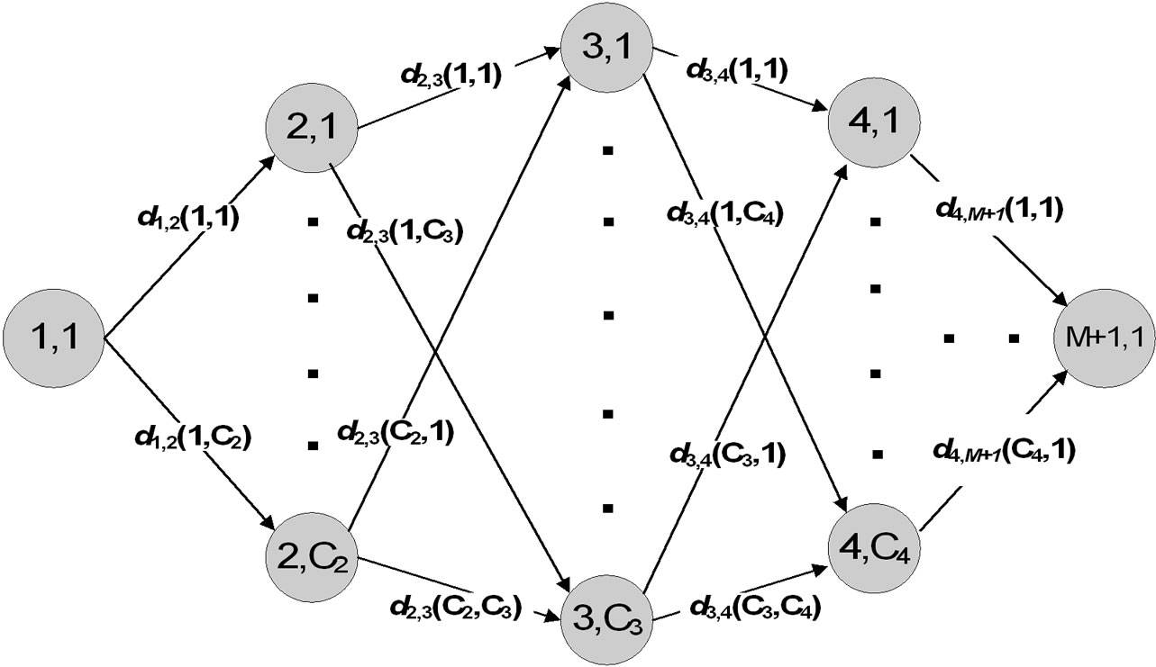
Figure 4. The CEP problem can be seen as the shortest path problem for an acyclic network in which the nodes represent all possible values of capacity points and the links represent CES values.
possible du,v values depends on the total number of capacity points; see Figure 4.
Suppose that all links (sub-problems) are calculated, the optimal solution for CEP can be found by searching for the optimal sequence of capacity points and their associated link state values. On that level the CEP problem can be seen as a shortest path problem for an acyclic network in which the nodes represent all capacity point values, and branches represent CES values; see Figure 4, Then Dijkstra’s algorithm or any similar algorithm can be applied.
The number of all possible du,v(au, av) values depends on the total number of capacity points. It is very important to reduce that number (Cp) and that can be done through imposing of appropriate capacity bounds or by introduction of adding constraints (e.g. max. delay). Through numerical test-examples we’ll see that many expansion solutions cannot be a part of the optimal expansion sequence.
4.1. Single Location Expansion Problem
Approach described in chapter above requires solving repeatedly a certain single location expansion problem (SLEP) in all possible modifications, looking for the best result. Let SLEPi,j (m, Di, ... Dj) be a Single Location Expansion Problem associated with link m for facility (capacity) type i, i+1, ... , j and corresponding values of capacity change intention Di, Di+1, ... , Dj .
For example, in solving SLEP1,3 for three different capacity types (bandwidth sub-pools) we have many expansion solutions divided into three different scenarios (expansion strategies):
a). capacity changes of one capacity type are not correlated with changes of others;
b). capacity changes of two capacity types depend on each other, but change of the third is independent;
c). capacity changes for all of three capacity types depend on each other.
From three expansion scenarios (expansion strategy) many different expansion solutions can be derived, depending on Di polarity. A lot of them are not acceptable and are not part of optimal sequence. For this problem an acceptable expansion solution has to satisfy some basic properties:
xi,m × Di,m ³ 0 (18)
yi,j,m × Di,m £ 0 (19)
yi,j,m× Dj,m ³ 0 (20)
Property (4.1.1) implies that the expansion (increase) of capacity type i cannot be acceptable if that facility has intention to be reduced on location (link) m (Di,m < 0). Similar stays for negative values.
Expansion (capacity increase) is also possible through conversion, so (18) and (19) imply the similar restriction as (20). Zero value of any capacity type means that any change of capacity is allowed. In scenario A. we have only one possible expansion solution. In scenario B. we can combine all three capacity types in couples. In scenario C. we can see that only one expansion solution exists. Totally, we have five different expansion solutions with many variations.
In scenarios B. and C. we have expansion solutions with conversions of capacity from one type to another. It can be done as stand-alone expansion or together with expansion. That means that the conversion is just complementary with the expansion in satisfying of traffic demands.
Conversions can be applied only when idle capacities are noticed or negative demand increments are present. Special case is occurred when conversion yi,j,m eliminates both: eliminating idle capacity of type i plus satisfying traffic demands of capacity type j. Also we can make distinction between two options: the partial expansion and the excessive expansion. The partial expansion xj,m means that demands are satisfied by expansion of appropriate capacity type j plus by conversion yi,j,m of capacity type i with higher quality level, but only if shortage of facility i is not occurred.
The excessive expansion means that the expansion amount xi,m is used to partially expand facility i and to satisfy demands for lower capacity type j, with conversion amount yi,j,m.
4.2. Adding Properties (the Improvement of CEP Algorithm)
The most of the computational effort is spent on computing of the sub-problem values. But a lot of expansion solutions are not acceptable and they cannot be a part of the optimal expansion sequence. The key for this very effective approach is in fact that extreme flow theory enables separation of these extreme flows which can be included in optimal expansion solution from those which cannot be. Any of du,v value, if it cannot be a part of the optimal sequence, is set to infinity. It can be shown that a feasible flow in the network given in Figure 3 corresponds to an extreme point solution of CEP if and only if it is not the part of any cycle (loop) with positive flows, in which all flows satisfy given properties; see [18]. One may observe that the absence of cycles with positive flows implies that each node has at most one incoming flow from the source node (positive or negative). This result holds for all single source networks. That means that optimal solution of du,v has at most one expansion (or reduction) for each facility.
Using a network flow theory approach, adding properties of extreme point solution are identified. These properties are used to develop an efficient search for the link costs du,v. Absence of such cycles with positive flows implies that extreme point solutions for CEP satisfy the following properties:
Ii,m × xi,m £ 0 (21)
Ii,m × yi,j,m ³ 0 (22)
Ij,m × yi,j,m £ 0 (23)
Ij,m × xi,m× yi,j,m = 0 if xi,m × yi,j,m ¹ 0 (24)
Ii,m × Ij,m × yi,k,m × yj,k,m = 0 if yi,k,m × yj,k,m ¹ 0 (25)
for: i, j , k = 1, 2 , 3 i ¹ k ¹ j ; m = 1, … , M+1 Properties (21) to (25) imply that the capacity of any capacity type is changed through an expansion, reduction or by conversion only if it doesn’t make cycles with positive flows.
(21) and (22) imply that the capacity of any capacity type can be increased by an expansion or by a conversion only if there is no idle capacity. Similar rule exists for reduction of idle capacity.
(23) implies that capacity can be reduced only if there is no capacity shortage.
(24) implies that incoming flow of facility, going to be converted (reduced) in partially or excessive expansion solution, has to be zero. If not, cycles with positive flows can be occurred; see Figure 5, on that diagram we have idle capacity from previous link (for first and second class). The third class is satisfied with capacity conversions
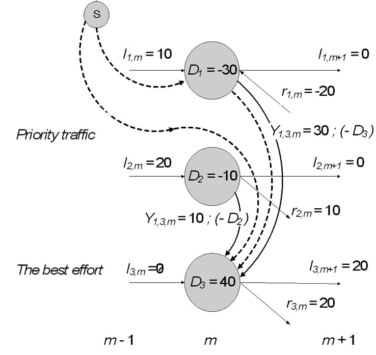
Figure 5. An example of single location expansion solution that cannot be a part of the extreme solution.
of higher classes. On that diagram dotted lines mark a cycle with positive flows from the common source. It means that such solution cannot be a part of extreme solution and has to be avoided from further calculation. One of the capacity values (I2,m or I3,m) must be zero.
Property (25) is used for simultaneous multiconversion solution from scenario C. Only one incoming flow of converted (reduced) facility can exist. It means that two incoming flows are not allowed in the same time. In the case of simultaneous conversions, incoming flows have to be zero.
We can say that any acceptable SLEP1,3 expansion solution for any CES have to satisfy properties (18)-(20) and (21)-(25). So many expansion solutions are not a part of optimal sequence and could be eliminated from further computation; see [19]. It means that any of subproblem value if it cannot be a part of the optimal sequence is set to infinity.
5. Testing Results and Comparison of Different Algorithm Options
The proposed algorithm is tested on many numerical test-examples, looking for optimal expansion sequence on the path. Between edge routers there are maximum M core routers (LSR) and the path consists of maximum M+1links. Traffic demands (former contracted SLAs) are given in relative amount for each interior router on the path. Demands are overlapping in time and are defined for each capacity type (service class). Results obtained by improved algorithm (reduction of unacceptable expansion solutions) are compared with results obtained by referent algorithm that is calculating all possible expansion solutions for each CES.
For each test-example we know the total number of
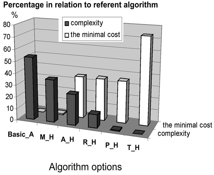
Figure 6. Trends of algorithm complexity and comparison of results (minimal cost).
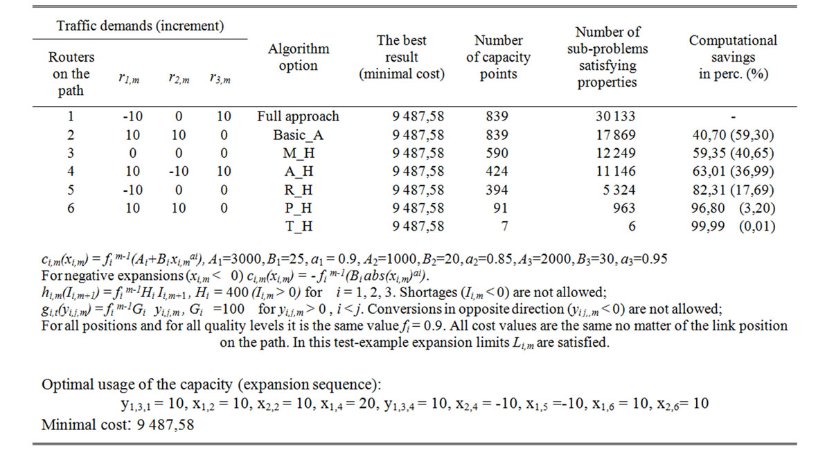
Table 1. Results of numerical test-example.
capacity points. The number of possible CES is wellknown, so it is the measure of the complexity for the CEPproblem. Also, for each test-example we can see the number of acceptable sub-problems, satisfying basic and additional properties of optimal flow; see example from table 1. For all numerical test-examples the best possible result (near-optimal expansion sequence) can be obtained with improved algorithm (denoted with Basic_A), same as with referent algorithm (without reduction of unacceptable expansion solutions). For N=3 and M=6 algorithm complexity savings in percents are on average more that 40 % that is proportionally reflected on computation time savings; see Figure 6.
The number of all possible CES values depends on the total number of capacity points. So CEP requires the computation effort of O(NMNd) with linear influence of N. In real application we normally apply definite granularity of capacity values through discrete values (integer) of traffic demands Ri . It reduces the number of the capacity points significantly. Because of that the minimal step of capacity change (step_Ii) has strong influence on the algorithm complexity.
In real situation we can introduce some limitations on the capacity state value, talking about heuristic algorithm options:
a) Only one negative capacity value in the capacity point. Such option is denoted with M_H (Minimal-shortage Heuristic option);
b) Total sum of the link capacity values (for all quality levels) is positive A_H (Acceptable Heuristic option);
c) Total sum is positive but only one value can be negative. Such option is denoted with R_H (Real Heuristic option);
d) Algorithm option that allows only non-negative capacity state values is denoted with P_H (Positive Heuristic option);
e) Only null capacity values are allowed. A trivial heuristic option (denoted with T_H) allows only zero values in capacity point (only one capacity point).
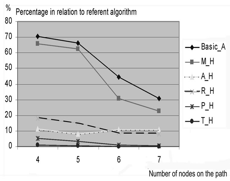
Figure 7. The complexity savings increase with value M.
We compared the efficiency of algorithm in above mentioned options. In Figure 6 we can see the average values of results for N=3 and M=6. Only for few test-examples (see table 1.) we can find the best expansion sequence, providing the minimal cost, no matter of algorithm option we use. For the most examples algorithm option M_H can obtain the best result with average saving more than 60 %. For other algorithm options the significant reduction of complexity is obvious but deterioration of result appears. In the most cases the trivial algorithm option (T_H) shows the significant deterioration of final result. A good fact for all algorithm options is that efficiency rises with increase of value M; see Figure 7.
6. Conclusions
Inappropriate bandwidth reservation or wrong traffic load could result in congestion possibilities. In this paper we propose an efficient algorithm for congestion control and load balancing purpose during SLA negotiation process.
We can check congestion probabilities on the path with algorithm of very low complexity first (e.g. P_H algorithm option). It means that only if congestion appears we need optimization with more complex algorithm (e.g. A_H). With the most complex algorithm option (Basic_A) we can get the best possible result, so we can be sure if congestion on the path could appear or not. In the case of congestion appearance new SLA cannot be accepted or adding capacity arrangement should be done. It means that SLA re-negotiation has to be done and customer has to change the service parameters: e.g. bandwidth (data speed), period of service utilization etc.
The proposed algorithm for load control (with different options) can be efficiently incorporated in SLA negotiation process. It may improve end-to-end provisioning, especially for overloaded and poorly connected networks where over-provisioning is not acceptable.
7. References
[1] F. L. Faucheur, et al., “Multi-protocol label switching (MPLS) support of differentiated services,” Technical Report RFC 3270, IETF, 2002.
[2] V. Sarangan and C. Jyh-Cheng, “Comparative study of protocols for dynamic service negotiation in the next-generation Internet,” IEEE Communication Magazine, Vol. 44, No. 3, pp. 151-156, 2006.
[3] N. Degrande, G. V. Hoey, P. L. V. Poussin, and S. Busch, “Inter-area traffic engineering in a differentiated services network,” Journal of Network and Systems Management (JNSM), Vol. 11, No. 4, 2003.
[4] M. D’Arienzo, A. Pescape, and G. Ventre, “Dynamic service management in heterogeneous networks,” Journal of Network and Systems Management (JNSM), Vol. 12, No. 3, pp. 349-370, 2004.
[5] K. Haddadou, S. G. Doudane, et al., “Designing scalable on-demand policy-based resource allocation in IP networks,” IEEE Communications Magazine, Vol. 44, No. 3, pp. 142-149, 2006
[6] R. Boutaba, W. Szeto, and Y. Iraqi, “DORA: Efficient routing for MPLS traffic engineering,” Journal of Network and Systems Management (JNSM), Vol. 10, No. 3, pp. 309-325, 2002.
[7] Y. Cheng, R. Farha, A. Tizghadam, et al., “Virtual network approach to scalable IP service deployment and efficient resource management,” IEEE Communication Magazines, Vol. 43, No. 10, pp. 76-84, 2005.
[8] S. Lima, P. Carvalho, and V. Freitas, “Distributed admission control for QoS and SLS management,” Journal of Network and Systems Management (JNSM), Vol. 12, No. 3, pp. 397-426, 2004
[9] J. Guichard, F. L. Faucheur, and J. P. Vasseur, “Definitive MPLS Designs,” Cisco Press, pp. 253-264, 2005.
[10] O. Younis and S. Fahmy, “Constraint-based routing in the internet: Basic principles and recent research,” IEEE Communications Surveys & Tutorials, Vol. 5, No. 1, pp. 2-13, 3rd quarter 2003.
[11] K. H. Ho, P. H. Michael, N. Wang, G. Pavlou, and S. Georgoulas, “Inter-autonomous system provisioning for end-to-end bandwidth guarantees,” Computer Communications, Vol. 30, No. 18, pp. 3757-3777, 2007.
[12] S. Bhatnagar, S. Ganguly, and B. Nath, “Creating multipoint-to-point LSPs for traffic engineering,” IEEE Communications Magazines, Vol. 43, No. 1, pp. 95-100, 2005.
[13] M. Morrow and A. Sayeed, “MPLS and next-generation networks: Foundations for NGN and enterprise virtualization, ” Cisco Press, 2006.
[14] S. Bakiras and L. Victor, “A scalable architecture for end-to-end QoS provisioning,” Computer Communications, Vol. 27, No. 13, pp. 1330–1340, 2004.
[15] S. Giordano, S. Salsano, and G. Ventre, “Advanced QoS provisioning in IP networks: The European premium IP projects,” IEEE Communication Magazines, Vol. 41, No. 1, pp. 30-36, 2003.
[16] D. Kagklis, C. Tsakiris, and N. Liampotis, “Quality of service: A mechanism for explicit activation of IP services based on RSVP,” Journal of Electrical Engineering, Vol. 54, No. 9-10, Bratislava, pp. 250-254, 2003.
[17] H. Luss, “A heuristic for capacity expansion planning with multiple facility types,” Naval Res. Log. Quart., Vol. 33, No. 4, pp. 685-701, 1986.
[18] W. I. Zangwill, “Minimum concavecost flows in certain networks,” Mgmt. Sci., Vol. 14, pp. 429-450, 1968
[19] S. Krile and D. Kuzumilovic, “The application of bandwidth optimization technique in SLA negotiation process,” Proceedings of 11th CAMAD’06, International Workshop on Computer-Aided Modeling, Analysis and Design of Communication Links and Net Network, Trento, pp. 115-121, 2006.
[20] S. Dasgupta, J. C. D. Oliveira, and J. P. Vasseur, “A new distributed dynamic bandwidth reservation mechanism to improve resource utilization: Simulation and analysis on real network and traffic scenarios,” Proceedings of 25th IEEE International Conference on Computer Communications INFOCOM, Barcelona, pp. 1-12, 2006.
[21] S. Dasgupta, J. C. D. Oliveira, and J. P. Vasseur, “Dynamic traffic engineering for mixed traffic on international networks,” Computer Networks, Vol. 11, pp. 2237 -2258, 2008.