Journal of Electromagnetic Analysis and Applications
Vol. 1 No. 4 (2009) , Article ID: 1123 , 4 pages DOI:10.4236/jemaa.2009.14042
Radio Wave Propagation Characteristics in FMCW Radar
![]()
Mathematics Department, Faculty of Science, Ain Shams University, Cairo, Egypt
Email: g_sami2003@yahoo.com
Received July 3rd, 2009; revised August 11th, 2009; accepted August 20th, 2009.
Keywords: Radio Wave, FMCW Radar, Cloud Profiling Radar
ABSTRACT
FMCW Radar (Frequency Modulated Continuous Wave Radar) is used for various purposes, such as atmospheric Remote Sensing, inter-vehicle ranging, etc. FMCW radar systems are usually very compact, relatively cheap in purchase as well as in daily use, and consume little power. In this paper, FMCW radar determines a target range by measuring the beat frequency between a transmitted signal and the received signal from the target, and Combines between PO and radar single. The approach based on frequency domain physical optics for the scattering estimation and the linear system modeling for the estimation of time domain response, and FMCW Radar signal processing.
1. Introduction
The FMCW radar has to adjust the range of frequencies of operation to suit the material and targets under investigation. The transceiver generates a signal of linearly increasing frequency for the frequency-sweep period. The signal propagates from the antenna to a static target and back. The value of the received-signal frequency compared to the transmitted-signal frequency is proportional to the propagation range. The main advantages of the FMCW radar are the wider dynamic range, lower noise figure and higher mean powers that can be radiated. In addition a much wider class of antenna is available for use by the designer.
The further advantage of FMCW radar is its ability to adjust the range of frequencies of operation to suit the material and targets under investigation if the antenna has an adequate pass-band of frequencies. This radar system mixes the wave reflected by a target object and part of the radiated wave to obtain a beat signal that contains distance and speed components. For large scatterer, the physical-optics approximation is an efficient method in the frequency domain [1,2]. This physical optics (PO) approximation is initially applied in the frequency-domain with the inverse Fourier transform [3], [4], [5], [6]. With FMCW, the high-frequency circuitry for beat signal detection is relatively simple and distance can be directly obtained. By mixing the received FMCW and transmitted FMCW signals, the system obtains a beat signal having a frequency f b.
2. The Principles of the FMCW Radar
The principle of the FMCW radar is shown in Figure 1. Transmitted signal from one of the antennas is reflected, and is received by the other antenna with delay time To relative to the original transmitted signal. Mixing the received and transmitted frequencies, the beat frequencies are observed in the spectra.
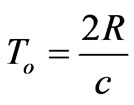
The time takes for the signal to travel the two-way distance between the target and the radar is To, hence [7], [8]:
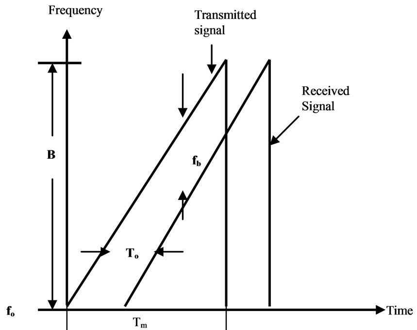
Figure 1. Principle of the FMCW radar
 (1)
(1)
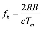
From the geometry of transmit and receive waveforms we can derive a relationship between the beat frequency f b, the range R, and c is the velocity of light.
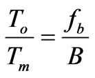
From Figure 1, we can see,
 (2)
(2)
Substituting (1) in (2), we get
 (3)
(3)
3. Scattered Wave from Radar Target
3.1 Frequency Domain Physical Optics
For a perfectly conducting body, the frequency-domain PO-induced current distribution over the illuminated surface is [9,10,11]:
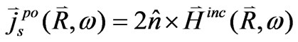 (4)
(4)
where  is the unit vector normal to the surface
  and
and  is the incident magnetic field with angular frequency w.
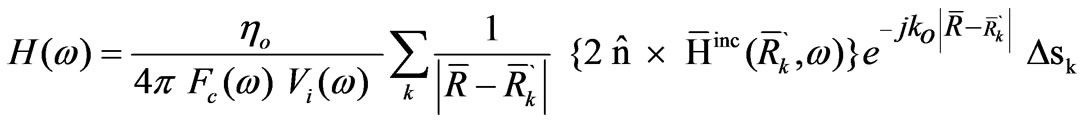
The frequency-domain scattered field is obtained by calculating the integral over the illuminated surface using the free space Green’s function:
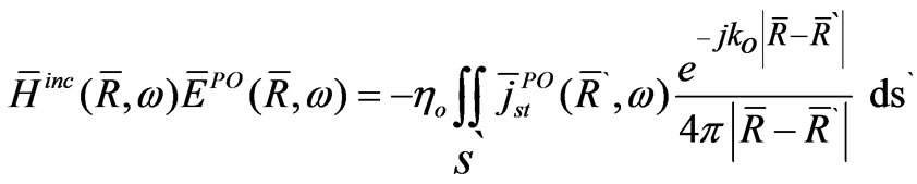 (5)
(5)
where the vector  locates the integration point on the scatterer surface,
  is the wave number,
 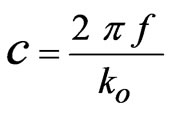 is the velocity of the light and
  is the intrinsic free space impedance, and
  is the surface-current distribution.
The frequency transfer function  is defined as
 (6)
(6)
where  is the input waveform in frequency domain physical optics, this is just a magnitude of the source.
The output Voltage  is calculated from
 by considering the receiver antennas as [12,13],
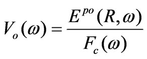 (7)
(7)
 (8)
(8)
where  is the Complex antenna factor.
3.2 Treatment of FMCW Signal
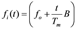
Instantaneous frequency fi(t), is given as
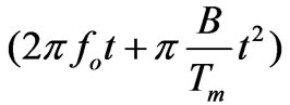
and the instantaneous phase , is defined as
 =
=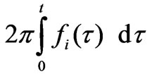 =
=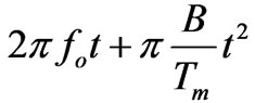 (9)
(9)
Using Equation (9), the FMCW signal waveform is defined as
 (10)
(10)
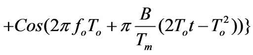
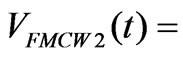
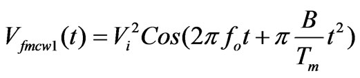
The output of mixer VFMCW1(t) is expressed as
 (11)
(11)
The output waveform vo(t) is vo(t) = vi(t )* h(t)
when h(t) is a sample delay of To, i.e.
h(t)= (12)
(12)
Therefore, mixer output signal is
 = vi (t) vi (t-To)(13)
where vi (t-To)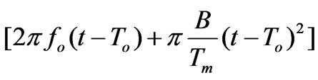
 (14)
(14)
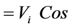
From Equations (10) and (11) we can calculate:
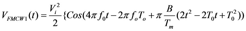
 (15)
(15)
The first Cos term describes a linearly increasing FM signal (chirp) at about twice the carrier frequency with a phase shift that is proportional to the delay time To. This term is generally filtered out.
The second Cos term:
 Cos
Cos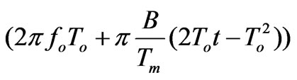 (16)
(16)
describes a beat signal at a fixed frequency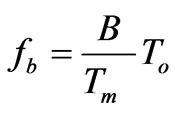 .
.
3.3 Combination of PO and Radar Single Processing
As h(t) given in section 3.2 is just an idealized model, more realistic h(t) obtained by PO in section 3.1, Equation (12) shall be used.
However, Equation (6) is given in frequency domain , and it shall be Inverse Fourier transformed
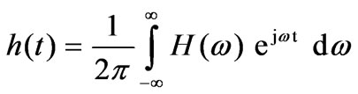 (17)
(17)
It is sufficient that  is computed only within the source frequency range, i.e.
 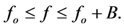 Outside the band,
  can be assumed zero,
  is also zero in this region.
In reality, Fourier transform shall be executed numerically. Let us assume the sampling interval  which shall satisfy the following relation
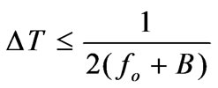 (18)
(18)
 (19)
(19)
 (20)
(20)
 (21)
(21)
where  is a sampling frequency,
  , and
, and  are some certain integers.
Now  is denoted as
 , and
, and  is given as,
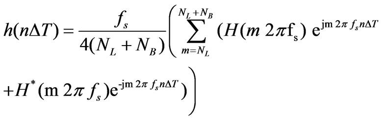 (22)
(22)
Convolution (11) is now implemented as,
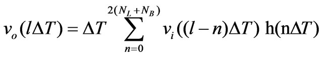 (23)
(23)
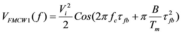
Substituting from (23) and (10) in (13), we can get
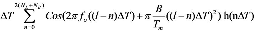 (24)
(24)
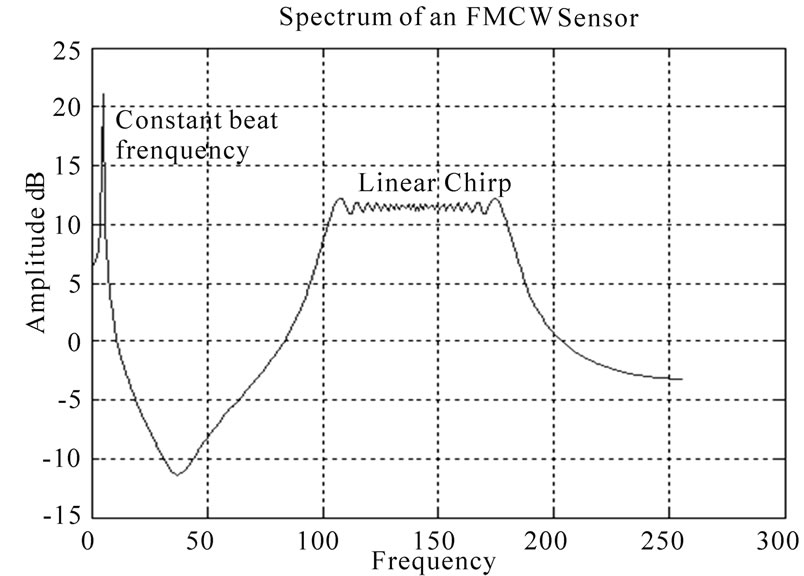
Figure 2. Frequency domain representation of FMCW sensor output
where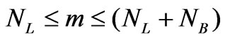 Now, we use Fourier Transformation, we get
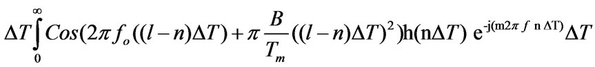
 (25)
(25)
And also we can get
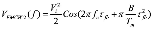 (26)
(26)
describes a beat signal at a fixed frequency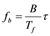 .
.
It can be seen that the signal frequency is directly proportional to the time delay time , and hence is directly proportional to the round trip time to the target.
4. Conclusions
This paper presents the time domain linear system analysis for FMCW radar response by performing the inverse Fourier transform over the frequency-domain scattered field which obtained by calculating the integral over the illuminated surface using the free space Green’s function. Then we got the received FMCW signal and transmitted FMCW signal, the product detection is implemented to get the beat signal. The Fourier transform is used to find the beat frequency.
REFERENCES
- W. V. T. Rusch and P. D. Potter, “Analysis of reflector antenna,” Academic, New York, pp. 46–49, 1970.
- R. F. Harrington, “Time-harmonic electromagnetic fields,” McGraw-Hill, New York, pp. 127, 1961.
- E. M. Kennaugh and R. L. Cosgriff, “The use of impulse response in electromagnetic scattering problems,” IRE Natl. Conv. Rec., Part 1, pp. 72–77, 1958.
- S. Hatamzadeh-Varmazyar and M. Naser-Moghadasi, “An integral equation modeling of electromagnetic scattering from the surfaces of arbitrary resistance distribution,” Progress In Electromagnetics Research B, Vol. 3, pp. 157–172, 2008.
- C. A. Valagiannopoulos, “Electromagnetic scattering from two eccentric Metamaterial cylinders with frequency-dependent permittivities differing slightly each other,” Progress In Electromagnetics Research B, Vol. 3, pp. 23–34, 2008.
- E. M. Kennaugh and D. L. Moffatt, “Transient and impulse response approximation,” Proceeding IEEE, pp. 893–901, August 1965.
- S. Hoshi, Y. Suga, Y. Kawamura, T. Takano, and S. Shimakura, “Development of an FMCW radar at 94 Ghz for observations of cloud particles-antenna section,” Proceeding of the Society of Atmospheric Electricity of Japan, No. 58, pp. 116, 2001.
- T. Takano, Y. Suga, K. Takei, Y. Kawamura, T. Takamura, and T. Nakajima, “Development of an cloud profiling FMCW radar at 94 Ghz, International Union of Radio Science,” General Assembly, Session FP, No. 1786, 2002.
- E. Yuan and W. V. T. Rusch, “Time-domain physical optics,” IEEE Transactions on Antenna and Propagation, vol. 42, no. 1, January 1994.
- L.-X. Yang, D.-B. Ge, and B. Wei, “FDTD/TDPO hybrid approach for analysis of the EM scattering of combinative objects,” Progress In Electromagnetics Research, PIER 76, pp. 275–284, 2007.
- G. M. Sami, “Time-domain analysis of a rectangular reflector,” Submitted.
- S. Ishigami, H. Iida, and T. Iwasaki, “Measurements of complex antenna factor by the Near 3-antenna method,” IEEE Transaction on Electromagnetic Compatibility, Vol. 38, No. 3, August, 1996.
- L. Li and C.- H. Liang, “Analysis of resonance and quality factor of antenna and scattering systems using complex frequency method combined with model-based parameter estimation,” Progress In Electromagnetics Research, PIER 46, pp. 165–188, 2004.