Int'l J. of Communications, Network and System Sciences
Vol.3 No.1(2010), Article ID:1180,7 pages DOI:10.4236/ijcns.2010.31013
An Evolutionary Algorithm Based on a New Decomposition Scheme for Nonlinear Bilevel Programming Problems
1School of Computer Science and Technology, Xidian University, Xi’an, China
2Department of Mathematics and Information Science, Qinghai Normal University, Xining, China
E-mail: lihecheng@qhnu.edu.cn
Received July 24, 2009; revised September 21, 2009; accepted November 4, 2009
Keywords: Nonlinear Bilevel Programming, Decomposition Scheme, Evolutionary Algorithm, Optimal Solutions
Abstract
In this paper, we focus on a class of nonlinear bilevel programming problems where the follower’s objective is a function of the linear expression of all variables, and the follower’s constraint functions are convex with respect to the follower’s variables. First, based on the features of the follower’s problem, we give a new decomposition scheme by which the follower’s optimal solution can be obtained easily. Then, to solve efficiently this class of problems by using evolutionary algorithm, novel evolutionary operators are designed by considering the best individuals and the diversity of individuals in the populations. Finally, based on these techniques, a new evolutionary algorithm is proposed. The numerical results on 20 test problems illustrate that the proposed algorithm is efficient and stable.
1. Introduction
The bilevel programming problem (BLPP) involves two optimization problems at different levels, in which the feasible region of one optimization problem (leader’s problem/upper level problem) is implicitly determined by the other (follower’s problem/lower level problem). The general bilevel programming problem can be formulated as follows.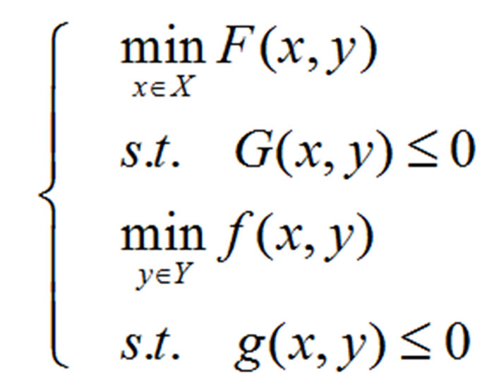
(1)
where  and
and  are called the leader’s and follower’s variables, respectively, F(f) :
  is called the leader’s (follower’s) objective function, and the vector-valued functions G :
  and g :
 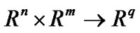 are called the leader’s and follower’s constraints, respectively; the sets X and Y place additional constraints on the variables, such as upper and lower bounds or integrality requirements etc. This mathematical programming model arises when two independent decision makers, ordered within a hierarchical structure, have conflicting objectives, and each decision maker seeks to optimize his/her objective function. In (1), the leader moves first by choosing a vector
  in an attempt to optimize his/her objective function F(x, y); the leader’s choice of strategies affects both the follower’s objective and decision space. The follower observes the leader’s choice and reacts by selecting a vector
  that optimizes his/her objective function f(x; y). In doing so, the follower affects the leader’s outcome.
BLPP is widely used to lots of fields such as economy, control, engineering and management [1,2], and more and more practical problems can be formulated as the bilevel programming models, so it is important to design all types of effective algorithms to solve different types of BLPPs. But due to its nested structure, BLPP is intrinsically difficult. It has been reported that BLPP is strongly NP-hard [2]. When all functions involved are linear, BLPP is called linear bilevel programming. It is the simplest one among the family of BLPPs, and the optimal solutions can occurs at vertices of feasible region. Based on these properties, lots of algorithms are proposed to solve this kind of problems [2–5]. When the functions involve nonlinear terms, the corresponding problem is called nonlinear BLPP, which is more complex and challenging than linear one. In order to develop efficient algorithms, most algorithmic research to date has focused on some special cases of bilevel programs with convex/concave functions[1,2,6–9], especially, convex follower’s functions [10–14]. In these algorithms, the convexity of functions guarantees that the globally optimal solutions can be obtained. Moreover, some intelligent algorithms, such as evolutionary algorithms (EAs)/ genetic algorithms (GAs) [10,15–17], tuba search approaches [18], etc, have been applied to obtain the optimal solutions to multi-modal functions. However, a question arises when the follower’s objective function is neither convex nor concave. On the one hand, it is difficult for us to obtain the globally optimal solution by using traditional optimization techniques based on gradients; on the other hand, if an intelligent algorithm, such as GA, is used to solve the follower’s problem, it can cause too large amount of computation [16]. To the best knowledge of the authors, there are not any efficient algorithm for this kind of BLPPs.
In this paper, we consider a special class of nonlinear BLPP with nonconvex objective functions, in which the follower’s objective is a function of the linear expression of all variables, and the follower’s constraints are convex with respect to the follower’s variables. There are no restrictions of convexity and differentiability on both the leader’s and the follower’s objective functions, which makes the model different from those proposed in the open literature. In view of the nonconvexity of the leader’s objective, we develop an evolutionary algorithm to solve the problem. First, based on the structural features of the follower’s objective, we give a new decomposition scheme by which the (approximate) optimal solution y to the follower’s problem can be obtained in a finite number of iterations. At the same time, the populations are composed of such points (x, y) satisfying the follower’s optimization problem, that is, y is an optimal solution of the follower’s problem when x is fixed, which improves the feasibility of individuals. Then, to improve the efficiency of proposed algorithm, the better individuals than crossover parents are employed to design new crossover operator, which is helpful to generate better offspring of crossover. Moreover, we design a singleside mutation operator, which can guarantee the diversity of individual in the process of evolution.
This paper is organized as follows. The model of the bilevel programming problem and some conceptions are presented in Section 2, and a solution method of the follower’s problem is given based on a decomposition scheme in Section 3. Section 4 presents an evolutionary algorithm in which new evolutionary operators are designed. Experimental results and comparison are presented in Section 5. We finally conclude our paper in Section 6.
2. Bilevel Programming Problem and Basic Notations
Let us consider the bilevel programming problem defined as follows
 (2)
(2)
where g(x, y) is convex and twice continuously differential in y, the function  is continuous,
 is vector-valued, where

 , and
, and 
 ,
, 

 , are all real constant. Now we introduce some related definitions and notations [2] as follows.
1) Search space: ;
;
2) Constraint region:
 ;
;
3) For x fixed, the feasible region of follower’s problem:
4) Projection of S onto the leader’s decision space:

5) For each , the follower’s rational reaction set:

6) Inducible region:
 .
.
In terms of aforementioned definitions, (2) can also be written as:

In order to ensure that (2) is well posed, in the remainder, we always assume that:
A1: S is nonempty and compact;
A2: For all decisions taken by the leader, each follower has some room to react, that is, .
.
A3: The follower’s problem has at most finite optimal solutions for each fixed x.
Since the leader’s functions may be nonconvex or nondifferential in (2), we use an evolutionary algorithm to solve the problem. However, due to the nested structure, the problem (2) always has a narrow inducible region (feasible region). If the individuals (x, y) are generated at random, there are large numbers of infeasible points in the populations, which makes the efficiency of EA decreased. To overcome the disadvantage, for x fixed, we first solve the follower’s problem to get the optimal solution y. After doing so, the point (x, y) at least satisfies or approximately satisfies the follower’s optimization. But the follower’s optimization problem may be nonconvex, how one can easily obtain the follower’s globally optimal solutions y for a fixed x? We finish the step in the next section
3. Solution Method of the Follower’s Problem
For any fixed x, we consider the follower’s problem of (2), that is,
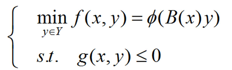 (3)
(3)
The optimal solutions to (3) can be found in several steps given as follows. Firstly, we solve the following nonlinear convex programming problems with linear objective function.
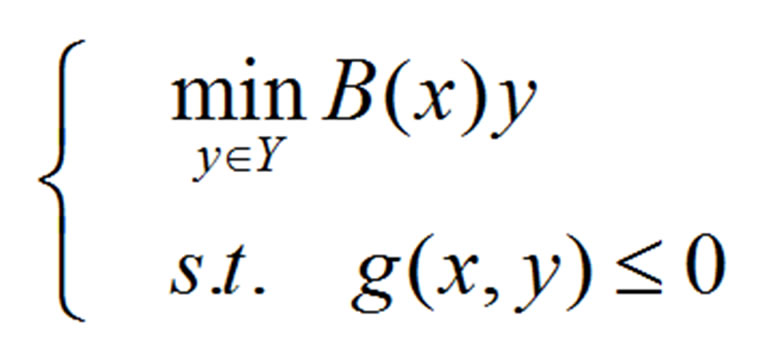 (4)
(4)
and
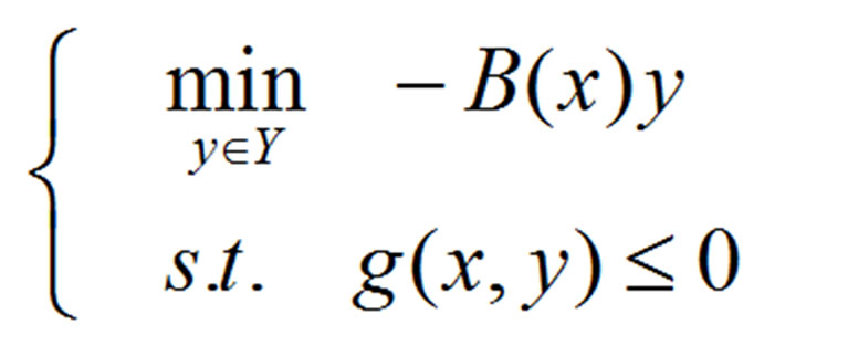 (5)
(5)
here, both (4) and (5) are convex programming problems, as a result, the optimal solutions can be obtained easily by the existing algorithms. We denote by ymin and ymax the optimal solutions to (4) and (5), respectively; setting B(x)ymin = a and B(x)ymax = b. In fact, we only need to consider the function  over the interval [a, b]. Secondly, let us find the monotone intervals of the function
  in [a, b], without any loss of generality, denote these intervals by [ai, bi]; i = 1, 2,…, k, and the index set corresponding to all increasing intervals is denoted by I1, while that corresponding to all decreasing intervals by I2. Thirdly, we consider the families of nonlinear programming problems as follows.
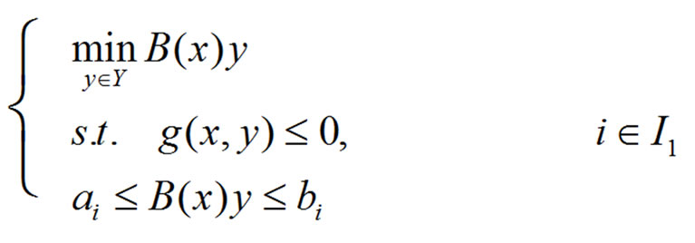 (6)
(6)
and
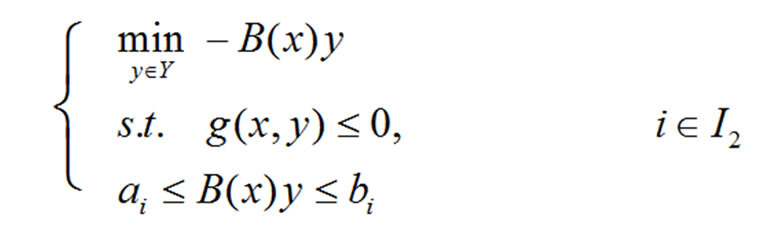 (7)
(7)
Evidently, the optimal solution to (3) can be obtained by solving (6) and (7). But it is computationally expensive to solve all of these nonlinear programming problems given by (6) and (7). In fact, we have Theorem 1. Each among (6) and (7) can get its minimum on the hyperplanes presented by B(x)y = , (
, ( = ai or bi, i = 1,2,…, k).
Proof. Note that B(x)y is linear with respect to y, as a result, it can achieve the minimum and maximum values at the boundary of S(x), and the two points were denoted by ymin and ymax. Let us recall that S(x) is convex, it follows that each point on the line segment yminymax is in S(x). Further, B(x)y is continuous in the compact set yminymax, it means for each![]() [a, b], there exists a point
[a, b], there exists a point  on yminymax such that B(x)
  =
= . As a result, it is easy to see that for each optimization problem presented by (6) and (7), there is a point satisfying B(x)y =
  in the feasible region. This completes the proof.
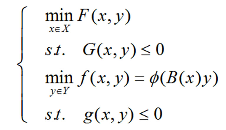
Since f(x, y) =  is constant over each hyperplane, we select a hyperplane on which f(x, y) has the smallest value. Recall assumption A3, there exists only a feasible point in the hyperplane. But how can one easily take the point from the hyperplane? Let us finish the process in the last step. Finally, draw a line segment connecting points ymin and ymax, which can be presented by the expression with a parameter t: y = ymin + t(ymax - ymin). One can obtain easily a feasible point on the hyperplane by considering both the expression and the equation of the hyperplane. If there are more than one optimal solution, that is, there exist several hyperplanes on which f(x, y) has the same smallest value, in terms of A3, the number of feasible points is finite in these hyperplanes, we can select one among them according to the fitness function values given in next section. The procedure of solving the follower’s problem is shown in Figure 1. In Figure 1, the elliptical region is the feasible region of the follower’s problem for some fixed x. In terms of the
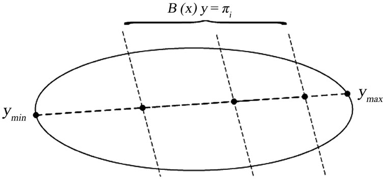
Figure 1. Follower’s feasible region and hyperplanes used to obtain the optimal value of .
.
monotonicity of , one can give the hyperplanes
 , and
, and  can achieve the optimal value on one or some hyperplanes. Also,
  is constant on each hyperplane, it means that the optimal solution of the follower’s problem can be found by checking the values of
  at the black points on
 .
.
4. Proposed Algorithm
In the section, we begin with the fitness function, crossover and mutation operators, and then propose an evolutionary algorithm with real number encoding to solve (2).
4.1. Fitness Function
Let us apply the penalty method to deal with the leader’s constraints. In order to use the technique efficiently, we design a dynamic parameter inspired by the sequential weight increasing factor technique (SWIFT) proposed by B. V. Sheela and P. Ramamoorthy [19]. The fitness function is denoted by F(x, y) + Mg
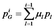
 . Where g stands for the generation number, Gi(x, y) are the components of G(x, y); Mg are penalty parameters (where M1 is given in advance as a positive constant, g = 1, 2,…) and computed as follows.
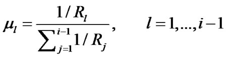
Choose n + 1 best points  from the current population. Let
Here , and
, and  is updated by the following formula.
 (8)
(8)
While n + 1 points chosen as above are affine independent, these points constitute a simplex 
 ; and
; and  as the generation number g increases.
4.2. Crossover Operator
Let N denote the population size. Rank all points in the population pop according to the fitness values from small to large. Without any loss of generality, we also denote these points by , and let
  > 0 stand for the fitness values of
 , i=1, 2 ,…, N. We give the crossover operator as follows.
Let  be a selected individual for crossover. The crossover offspring
  of the individual is got as follows.
 (9)
(9)
where  is random,
  is a positive constant,
  is arbitrarily chosen in the current population and
In the designed crossover operator, all better individuals than the crossover parent are used to provide a good direction for crossover, and the coefficients  make
make  closer to the points with smaller fitness.
4.3. Single-Side Mutation Operator
Let  be a parent individual for mutation. The mutation offspring
  of
of  is generated as follows.
At first, to select a component  of
of  at random, then the hyperplane
  divides the search space X into two hypercubes. Let
  represents the hypercube in which any point satisfies
  while
while  stands for the other,
  presents the volume of
  (
( ); and
  represents the set of all individuals belonging to
 ,
,  stands for the set of other points in the population;
  presents the number of elements in the set W. Then
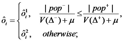 (10)
(10)
where  is a point taken randomly in
  (
( );
); is a small positive number, which keeps the denominators away from zero.
The mutation operator designed so is helpful to uniformly generate points in X, which can help to prevent the algorithm from the premature convergence.
4.4. Evolutionary Algorithm Based on the New Decomposition Scheme (EABDS)
Step 1. (Initialization) Randomly generate N initial points . For each
  fixed, we solve the follower’s problem for yi via the algorithm presented in Section 3. All of the points (
 ) form the initial population pop(0) with population size N. Let k = 0;
Step 2. (Fitness) Evaluate the fitness value R(x, y) of each point in pop(k);
Step 3. (Crossover) Randomly select a parent (x, y) from pop(k) according to the crossover probability . We first execute the crossover for the component x of the parent, and denote the offspring by
 . For fixed
 , the follower’s problem is solved to get the optimal solution
 . Then we can obtain a crossover offspring (
 ). Let O1 stand for the set of all these offspring;
Step 4. (Mutation) Randomly select parents from pop(k) according to the mutation probability . For each selected parent (x, y), we first execute the mutation for x and get its offspring
 , then for fixed
 , we optimize the follower’s problem for
 . (
. (![]() ) is the mutation offspring of (x, y). Let O2 represent the set of all these offspring.
) is the mutation offspring of (x, y). Let O2 represent the set of all these offspring.
Step 5. (Selection) Let . We evaluate the fitness values of all points in O, select the best N1 points from the set
  and randomly select
  points from the remaining points of the set. These selected points form the next population pop(k + 1);
Step 6. If the termination condition is satisfied, then stop; otherwise, let k = k+1, go to Step 3.
5. Simulation
We select 14 test problems from the references [4,7,8,10, 12–15,17]. All problems are nonlinear except for g01, g02, g05, and g08. In these problems, the function involved is differentiable and convex. In order to test the effectiveness of the proposed algorithm for nonconvex or nondifferentiable problems, we also construct 6 additional test problems as follows.
We first choose 2 test problems g10 and g08 randomly from the 14 problems:
g10) 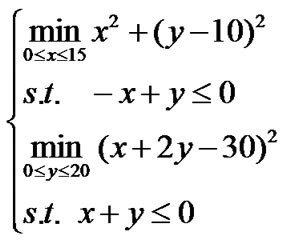
g08)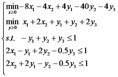
and replace the follower’s objective functions of the two problems by new constructed ones, respectively. As a result, we get problems g15-g20, in which problems g15- g17 are the same as problem g10 except for g15)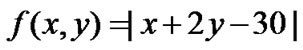 ;
;
g16)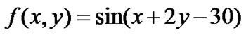 ;
;
g17)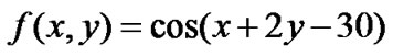 ;
;
While problems g18 -g20 have the same functions as problem g08 except for g18) 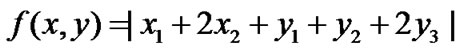
g19) 
g20) 
Generally speaking, the functions constructed so are nondifferentiable or nonconvex, which makes the corresponding BLPPs more difficult to solve than those with differentiable and convex objective functions.
The parameters are chosen as follows: the population size N = 30, the crossover probability pc = 0.8, the mutation probability pm = 0.2, N1 = 20,  = 2 and M1 = 100. For g01- g20, the algorithm stops when the best result can not be improved in 20 successive generations or after 50 generations. We execute EABDS in 30 independent runs on each problem on a computer (Intel Pentium IV-2.66GHz), and record or compute the following data:
1) Best values ( ), worst values (
 ), mean (
 ), median (
 ) and standard deviation (Std) of the objective function values in all 30 runs.
2) Best solutions ( ) in all 30 runs.
3) Mean of generation numbers ( ), and mean numbers of the individuals (MNI) used by EABDS.
All results are presented in Tables 1-2, in which Table 1 provides the comparison of the results found by both EABDS and the compared algorithms for problems g01-g20. Table 2 shows the best solutions found by both EABDS and the algorithms in the related references for g01-g20, and  and CPU used by EABDS are provided in Table 2. NA means that the result is not available for the algorithms, ‘*’ presents the problem is the maximization model and Ref stands for the related algorithms in references in Tables 1-2.
It can be seen from Table 1 that for problems g01, g03, g05, g07 [13,17], g08 [17], g09 [15] and g10, the best results found by EABDS are much better than those by the compared algorithms in the references, which indicates the algorithms in the related conferences can’t find the globally optimal solutions of these problems. For the constructed problems g15-20, EABDS gives uniform results. From the constructed objective functions, one can easily see that g15 has the same optimal solutions as g10, and g18 has the same optimal solutions as g08, which is also illustrated by the computational results in Tables 1,2. This means that EABDS can be used to solve nonlinear BLPPs with the nondifferentiable and noncom
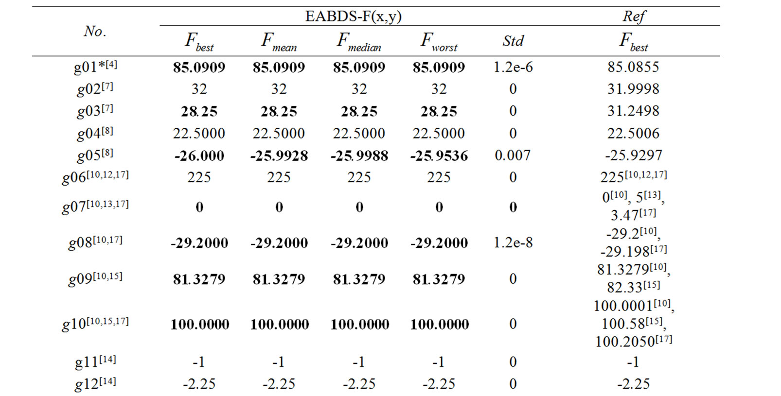
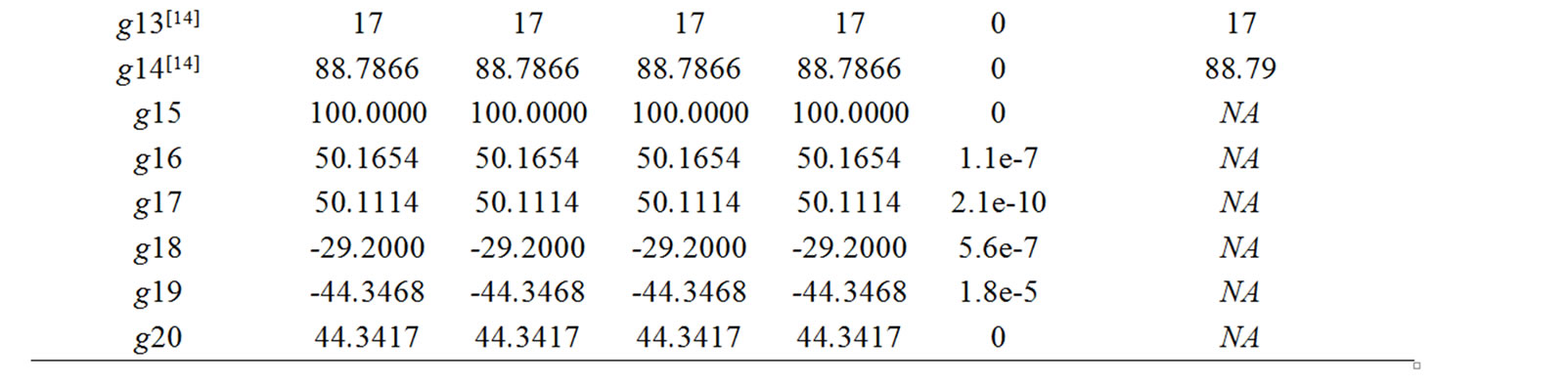
Table 1. Comparison of the best results found by EABDS and the algorithms presented by related references.
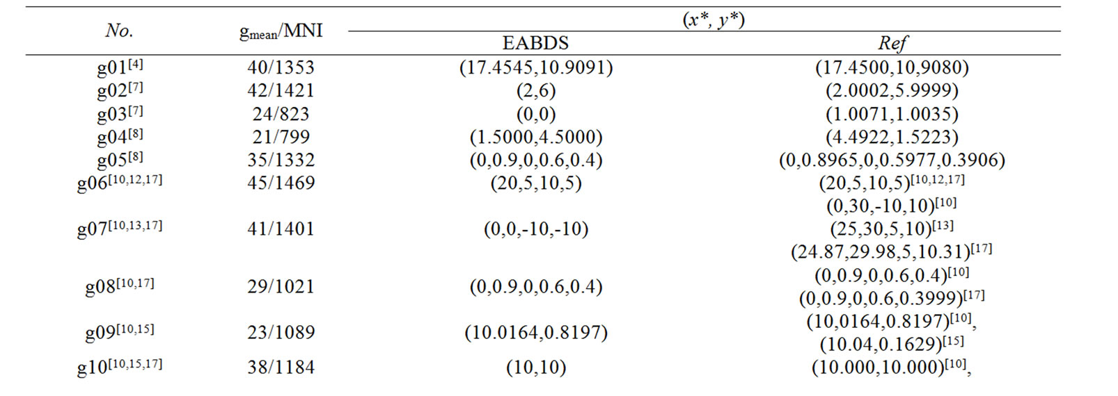
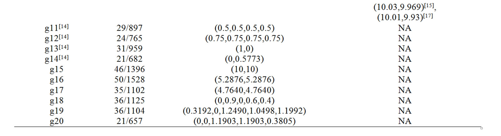
Table 2. Comparison of the solutions found by EABDS and the related algorithms in references, gmean and MNI needed by EABDS.
vex follower’s functions. For other problems except for g02, the best results found by EABDS are almost as good as those by the compared algorithms. For g02, although the result found by EABDS is a little bit worse than that by the compared algorithm, it should be noted that [7] provides an approximate solution of the follower’s problem, which makes the result better than that by EABDS, in fact, EABDS provides a precise solution. In all 30 runs, EABDS finds the best results of all problems except for problems g01, g05, g08 and g16-g19. For these problems, from Table 1, we can find the worst results are close to the best results and the standard deviations are also very small. This means that EABDS is stable and robust.
From Table 2, we can also see that for all of the problems, EABDS needs much less MNI and gmean, which means the proposed algorithm is efficient.
6. Conclusions
For the nonlinear bilevel programming problems with a special follower’s objective, we propose an evolutionary algorithm based on a decomposition scheme, in which based on the best points generated so far, we design a new crossover operator, and apply the approximate SWIFT to deal with the leader’s constraints. From the data simulation, we can also see easily that the proposed algorithm is especially effective and efficient for solving this kind of BLPPs.
7. Acknowledgment
This work was supported by the National Natural Science Foundation of China (No. 60873099).
8. References
[1] B. Colson, P. Marcotte, and G. Savard, “Bilevel programming: A survey,” A Quarterly Journal of Operations Research (4OR), Vol. 3, pp. 87–107, 2005.
[2] J. F. Bard, “Practical bilevel optimization,” The Netherlands: Kluwer Academic Publishers, 1998.
[3] U. P. Wen and S. T. Hsu, “Linear bi-level programming problems-A review,” The Journal of the Operational Research Society, Vol. 42, pp. 125–133, 1991.
[4] K.-M. Lan, U.-P. Wen, H.-S. Shih, et al., “A hybrid neural network approach to bilevel programming problems,” Applied Mathematics Letters, Vol. 20, pp. 880–884, 2007.
[5] H. I. Calvete, C. Gale, and P. M. Mateo, “A new approach for solving linear bilevel problems using genetic algorithms,” European Journal of Operational Research, Vol. 188, pp. 14–28, 2008
[6] L. D. Muu and N. V. Quy, “A global optimization method for solving convex quadratic bilevel programming problems,” Journal of Global Optimization, Vol. 26, pp. 199–219, 2003.
[7] D. L. Zhu, Q. Xua, and Z. H. Lin, “A homotopy methodfor solving bilevel programming problem,” Nonlinear Analysis, Vol. 57, pp. 917–928, 2004.
[8] H. Tuy, A. Migdalas, and N. T. Hoai-Phuong, “A novel approach to bilevel nonlinear programming,” Journal of Global Optimization, Vol. 38, pp. 527–554, 2007
[9] H. I. Calvete and C. Gale, “On the quasiconcave bilevel programming problem,” Journal of Optimization Theory and Applications, Vol. 98, pp. 613–622, 1998.
[10] Y. P. Wang, Y. C. Jiao, and H. Li, “An evolutionary algorithm for solving nonlinear bilevel programming based on a new constraint - handling scheme,” IEEE Trans. on Systems, Man, and Cybernetics-Part C, Vol. 35, pp. 221– 232, 2005.
[11] H. C. Li and Y. P. Wang, “A hybrid genetic algorithm for solving a class of nonlinear bilevel programming problems,” Proceedings of Simulated Evolution and Learning- 6th International Conference, SEAL, pp. 408–415, 2006.
[12] K. Shimizu and E. Aiyoshi, “A new computational method for Stackelberg and minmax problems by use of a penalty method,” IEEE Transactions on Automatic Control, Vol. 26, pp. 460–466, 1998.
[13] E. Aiyoshi and K. Shimizu, “A solution method for the static constrained Stackelberg problem via penalty method,” IEEE Transactions on Automatic Control, Vol. AC-29 (12), pp. 1111–1114, 1984.
[14] B. Colson, P. Marcotte, and G. Savard, “A trust-region method for nonlinear bilevel programming: algorithm & computational experience,” Computational Optimization and Applications, Vol. 30, pp. 211–227, 2005.
[15] V. Oduguwa and R. Roy, “Bilevel optimization using genetic algorithm,” Proceedings of IEEE International Conference on Artificial Intelligence Systems, pp. 123– 128, 2002.
[16] B. D. Liu, “Stackelberg-Nash equilibrium for mutilevel programming with multiple followers using genetic algorithms,” Computer mathematics Application, Vol. 36, No. 7, pp. 79–89, 1998.
[17] X. B. Zhu, Q. Yu, and X. J. Wang, “A hybrid differential evolution algorithm for solving nonlinear bilevel programming with linear constraints,” Proceedings of 5th IEEE International Conference on Cognitive Informatics (ICCI’06), pp. 126–131, 2006.
[18] J. Rajesh, K. Gupta, and H. Shankar, et al., “A tabu search based approach for solving a class of bilevel programming problems in chemical engineering,” Journal of Heuristics, Vol. 9, pp. 307–319, 2003.
[19] B. V. Sheela and P. Ramamoorthy, “SWIFT-S new constraines optimization technique,” Computer Methods in Applied Mechanics and Engineering, Vol. 6, pp. 309–318, 1975.