Journal of Biomedical Science and Engineering
Vol.6 No.1(2013), Article ID:27659,8 pages DOI:10.4236/jbise.2013.61013
Analytical image reconstruction methods in emission tomography
![]()
Department of Physics, Faculty of Sciences, University of Guilan, Rasht, Iran
Email: nooriasl.mahsa@gmail.com
Received 11 November 2012; revised 13 December 2012; accepted 20 December 2012
Keywords: Image Reconstruction; Fourier Transform; Back-Projection; Filtering
ABSTRACT
Data collected in two-dimensional projections give planar images of object at each projection angle. To obtain information along the depth of the object, tomographic images are reconstructed using these projections. There are basically two approaches to solve the problem of reconstruction: analytical and iterative, each one presenting its own advantages and limitations. This paper provides a detailed introduction and comparison to four analytical image reconstruction methods including Fourier transformation, simple backprojection, back-projection filtering and filtered backprojection.
1. INTRODUCTION
The basic problem of reconstruction in emission tomography is to estimate a volumetric radioactive distribution from a set of two-dimensional projections (camera based acquisitions in SPECT) or a set of lines of response (ring detectors based acquisitions in PET).
The reconstruction methods are divided into analytic and iterative approaches, each one presenting its own advantages and limitations. The choice of one or the other depends basically on the clinical objective of the study and the computational facilities supplied by the imaging system manufacturers. Analytic reconstruction methods offer a direct mathematical solution for the formation of an image. Iterative methods are based on a more complicated mathematical solution requiring multiple steps to arrive at an image.
We are considering four analytical image reconstruction methods here. Firstly, the Fourier transformation method that estimate the distribution by inverting Fourier transform theorem. Secondly, the simple back projection method that is just reverse of the projection operation which gave rise to the data. Thirdly, the back-projection filtering (BPF) method where the projection data are first back-projected, filtered in Fourier space and finally, the filtered back-projection (FBP) method where projection data are first filtered and then back projected (i.e., just reverse BPF method).
2. BISIC CONCEPTIONS OF RECONSTRUCTION
2.1. Projection and Sinogram
In SPECT, as a gamma-camera rotates in small steps around a patient, it creates a series of planar images called projections. At each stop, only photons moving perpendicular to the camera face pass through the collimator. A SPECT study consists of many planar images acquired at various angles.
In PET, two-dimensional imaging only considers lines of response (LORs) lying within a specified imaging plane. The acquired data are collected along LORs through a two-dimensional object as indicated in Figure 1. The LORs are organized into sets of projections, line integrals for all  for a fixed direction θ [1].
The collection of all projections for 0 ≤ θ < 2π forms a two-dimensional function of  and θ that is called a sinogram. The projection data of each slice along the axis of the gamma camera (i.e. the axis of rotation) is stored in an individual sinogram, where each row corresponds to one projection. Different rows represent different projection angles. This sinogram is aptly named because a fixed point in the object traces a sinusoidal path in the projection space. A sinogram for a general object will be the superposition of all sinusoids corresponding to each point of activity in the object as shown on the right of Figure 1.
The aim of the reconstruction process is to retrieve the radiotracer spatial distribution from the projection data.
2.2. Radon Transform Theorem
Mathematically a projection can be described by the Radon transform theorem. This theorem, supposed by Radon, states that image reconstruction from projections is possible [2,3]:
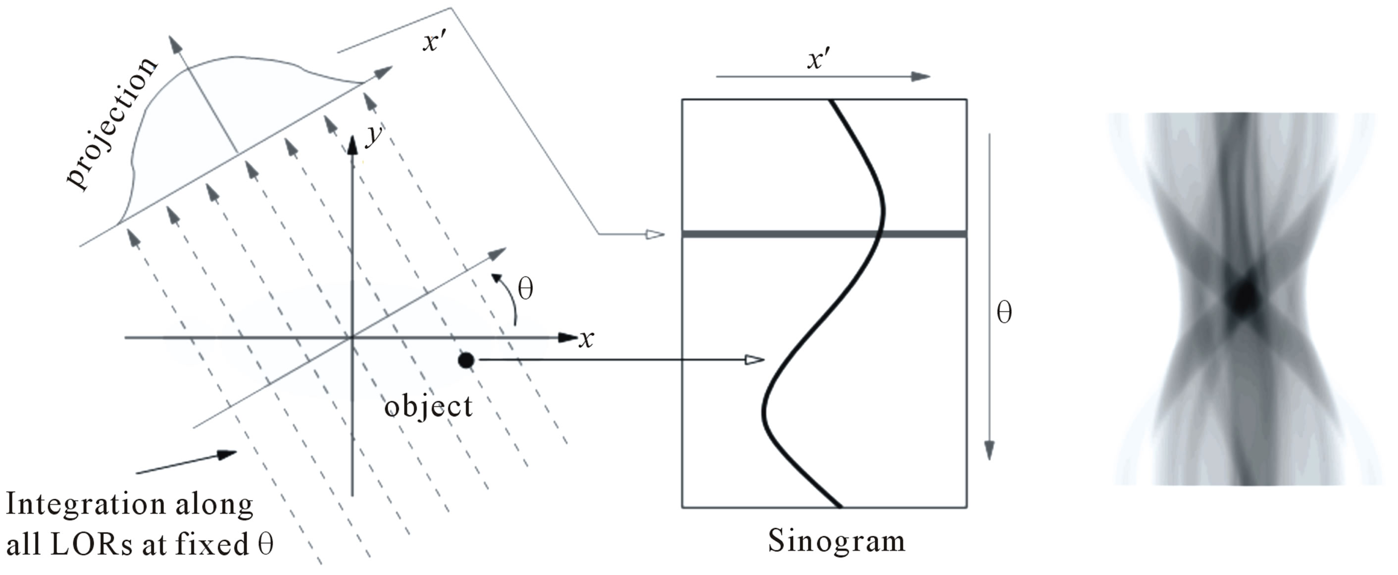
Figure 1. Illustration of a projection and a sinogram. The projections are organized into a sinogram such that each complete projection fills a single row of θ in the sinogram. A sinogram for a general object is shown on the right.
“The value of a two-dimensional function at an arbitrary point is uniquely obtained by the integrals along the lines of all directions passing the point”.
The Radon transformation shows the relationship between the two-dimensional object and the projections and guarantees that a two-dimensional object is reconstructed from projections obtained by the rotational scanning.
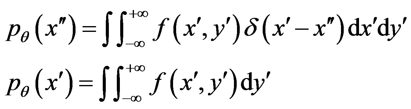
Radon transform is a projective transformation of a two-dimensional function onto the polar coordinate space  (see Figure 2) and is given as:
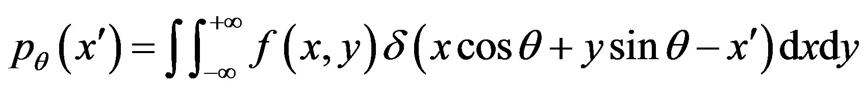 (1)
(1)
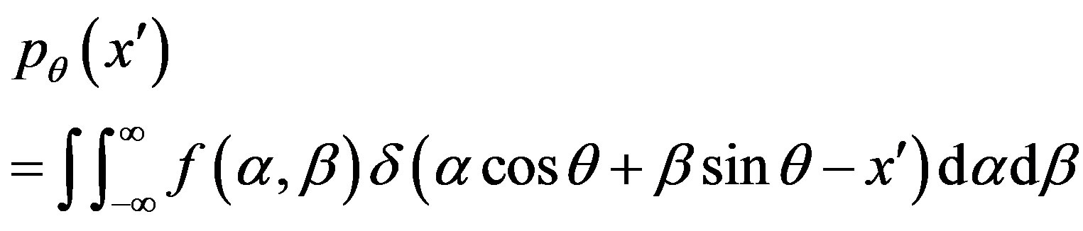
where  is a projection of
  on the axis
  of θ direction. The function
  is obtained by the integration along the line whose normal vector is in θ direction.
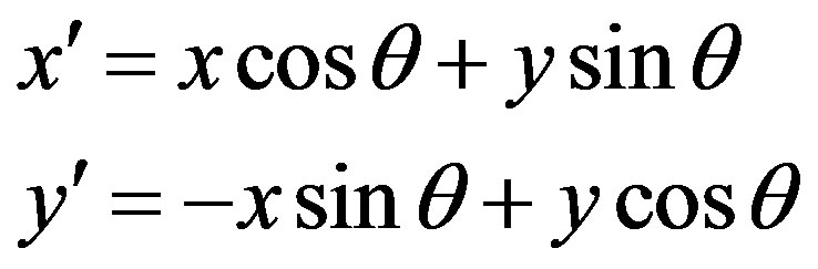
Although the Radon transformation expresses the projection by the 2-D integral on the  -coordinate, the projection is more naturally expressed by an integral of one variable since it is a line integral. Since the
  -coordinate along the direction f projection is obtained by rotating the
  -coordinate by θ, the relationship between two directions is expressed as follows:
 (2)
(2)
Since the translation from the  -coordinate to the
  -coordinate yields no expansion or shrinkage, we get
 . Then,
 (3)
(3)
2.3. The Fourier Slice Theorem (Central Projection Theorem)
The 1-D Fourier transformation of the projection is [4,5]:
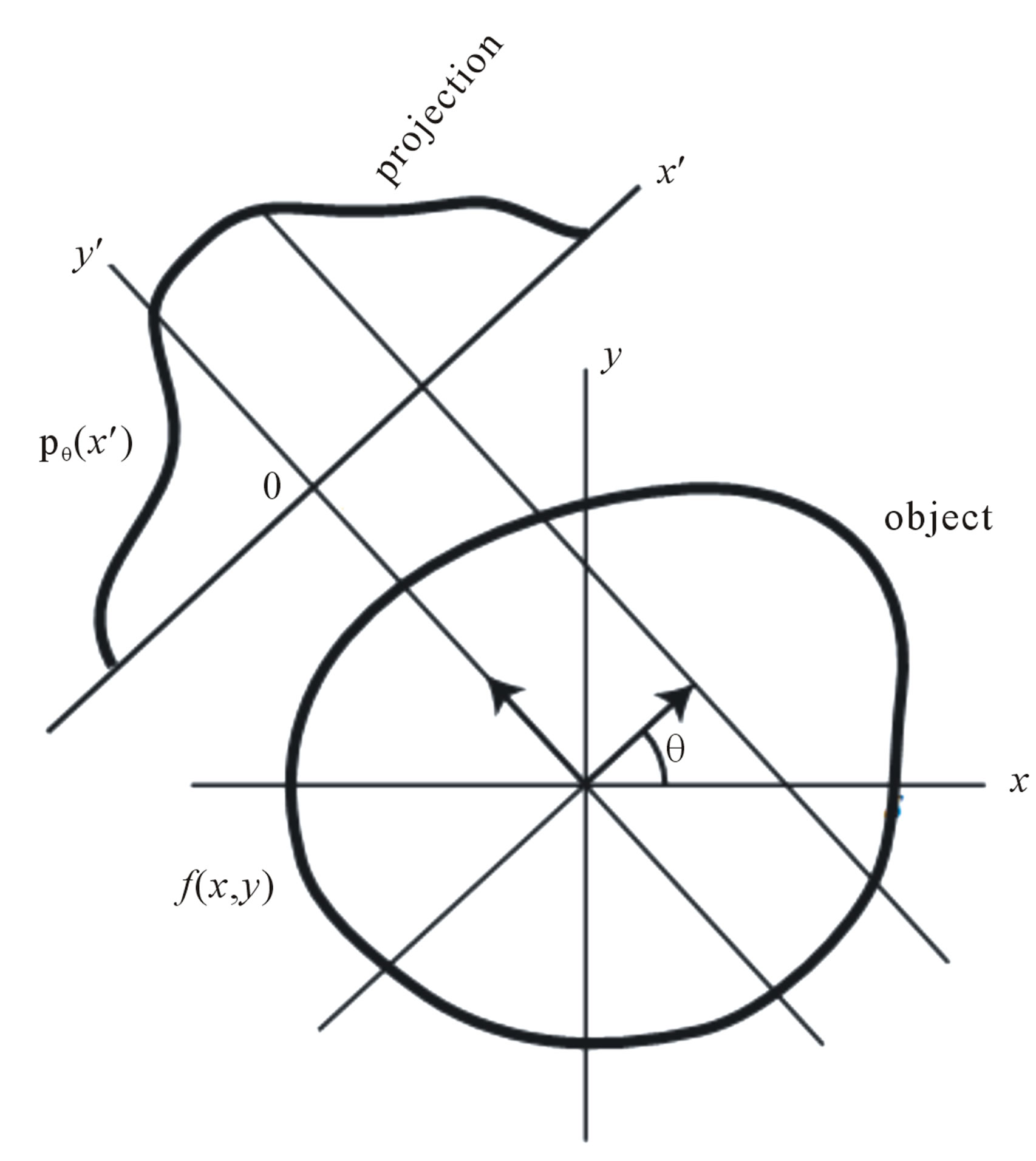
Figure 2. Illustration for Radon transform theorem.
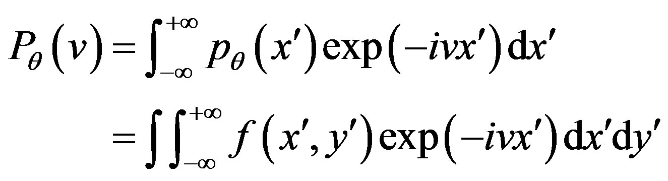 (4)
(4)
employing of Eq.2:
 (5)
(5)
In the next step, we calculate the 2-D Fourier transform of ,
, :
:
 (6)
(6)
transforming to polar coordinates,  , in the Fourier domain,
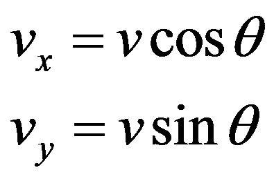
we get,
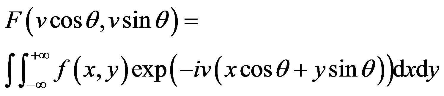 (7)
(7)
comparing Eqs.5 and 7, we result:
 (8)
(8)
The last equation states that the 1-D Fourier transform of the projection , denoted
 , is identical to the cross-section of the 2-D Fourier transform of the object
 , perpendicular to the direction of the projection, denoted
 . This important result is known as the Fourier slice theorem or the central projection theorem and is illustrated in Figure 3.
3. IMAGE RECONSTRUCTION METHODS
3.1. The Fourier Transformation (FT) Method
The Fourier slice theorem [3] indicates that the projection at an angle θ yields one cross-section of the Fourier transform of the original object, . Thus the projections for all θ yield the whole profile of
  (see Figure 3). The inverse Fourier transformation of
  yields the full reconstruction of
 . This reconstruction method is called Fourier transformation method. A scheme of this reconstruction has showed in Figure 4.
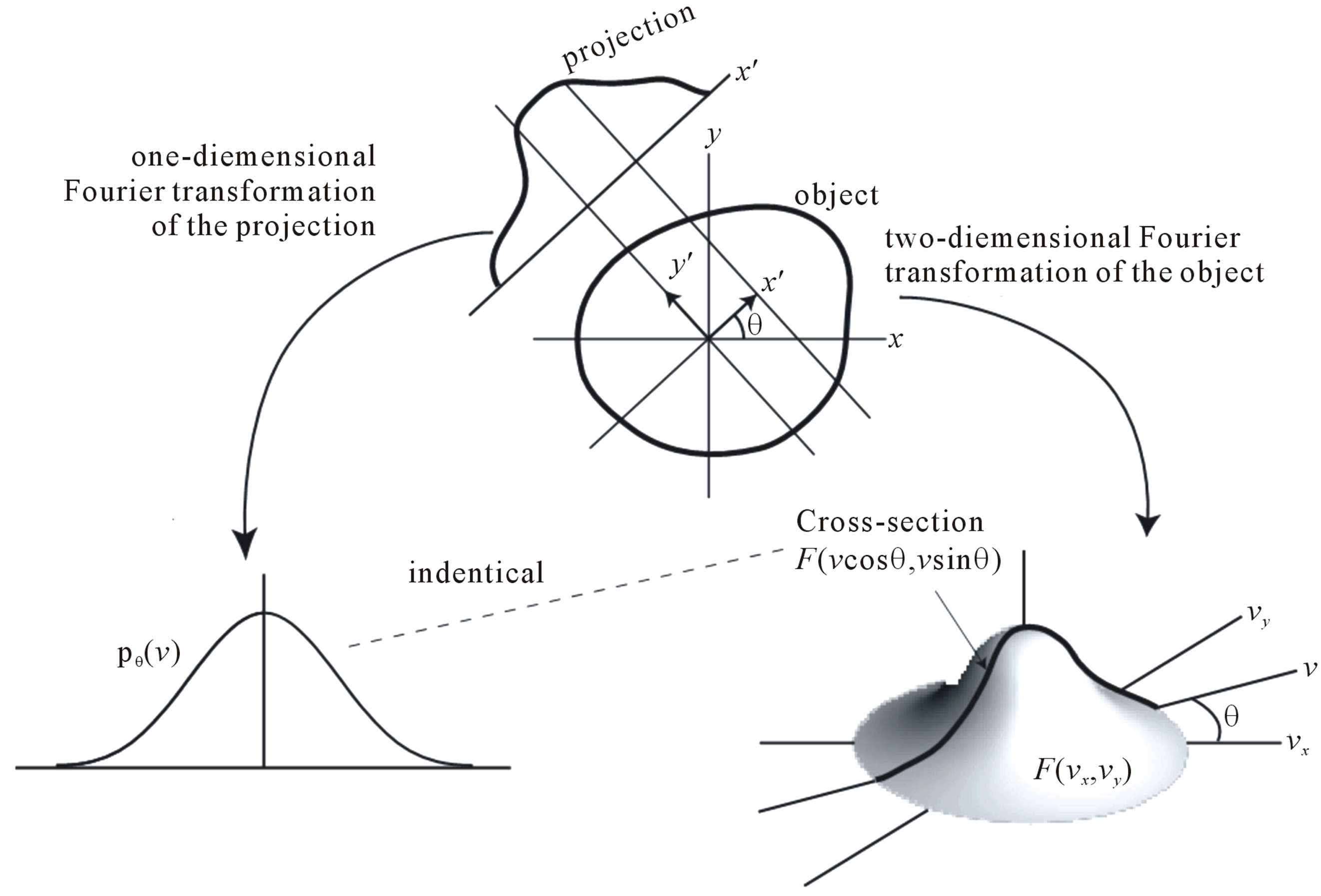
Figure 3. Illustration of Fourier slice theorem.
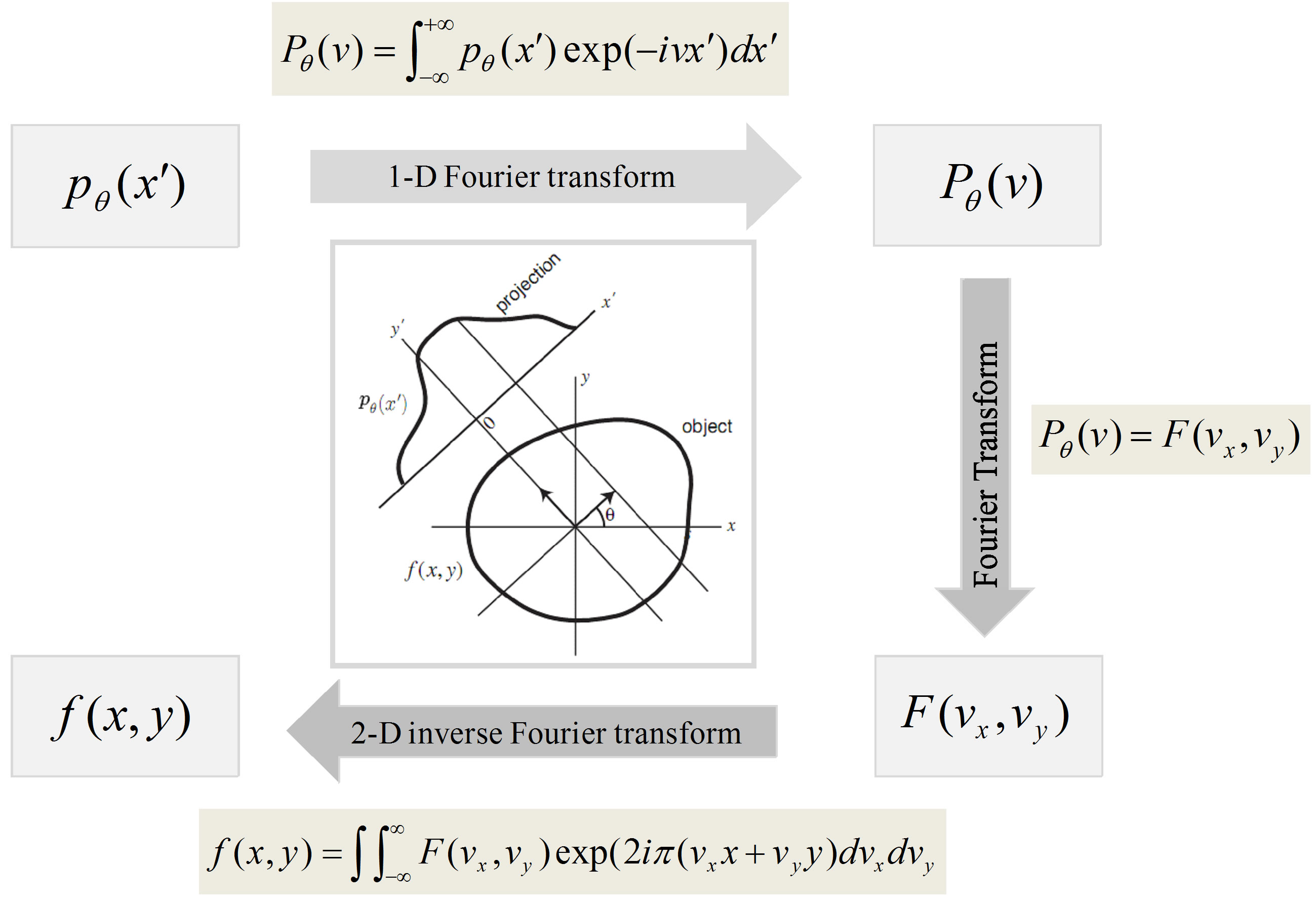
Figure 4. Flow of direct Fourier transform reconstruction.
3.2. The Simple Back-Projection (BP) Method
In this reconstruction method, to reconstruct , which is the absorbance at point
 , we consider the summation of projections passing through
  for all θ. Since these projections are line integrals through
 , it is duplicated and enhanced in the summation. Thus
  is reconstructed by this summation although it contains blur by absorbances at other points included in the projections. This reconstruction method is called simple back-projection (BP) method [5].
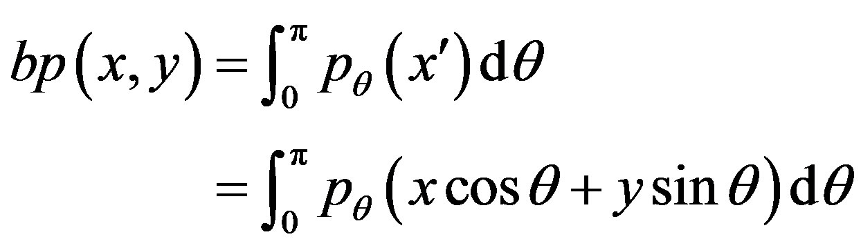
Based on this method, the summation of  for all θ yields the reconstructed image by the back-projection method, denoted
 , i.e.
 (9)
(9)
substituting the definition of the Radon transformation (Eq.1), we get
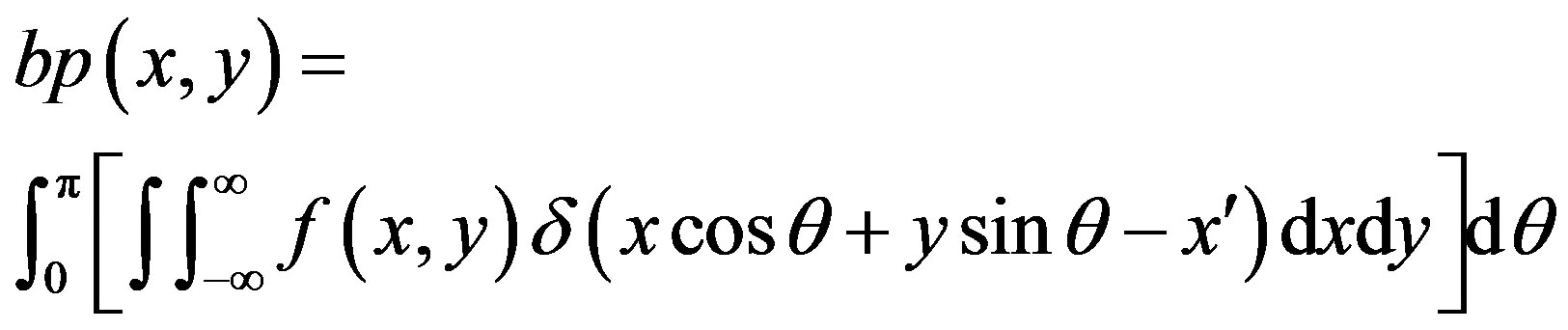 (10)
(10)
To prevent confusion, we change  -variables to
  before submitting
 ,
,
 (10′)
(10′)
After  from Eq.2 submitted into Eq.10′, we get
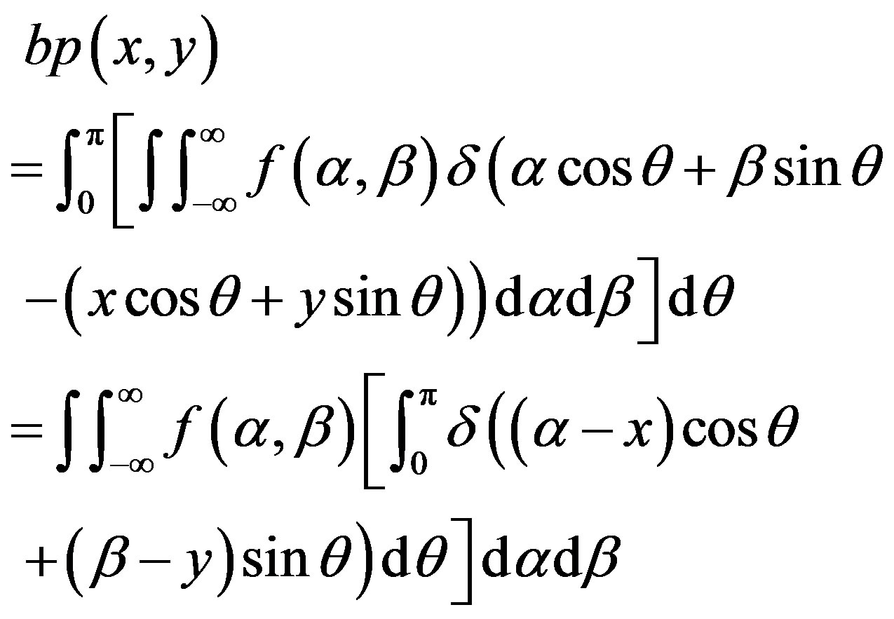 (11)
(11)
assuming,
we get,
 (12)
(12)
Now, rewriting term into the Dirac delta function in Eq.11 using of Eq.12, we can employ the following theorem,
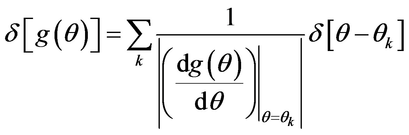 (13)
(13)
According to Eq.13,  for a finite number of
 . This obtain to submit
  in Eq.12 that result
 . Then submitting this value for
  in Eq.13, we get
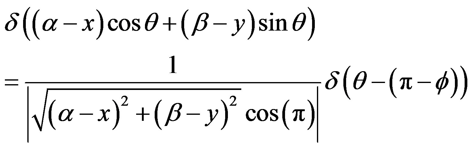 (14)
(14)
submitting Eq.14 into Eq.11, we get
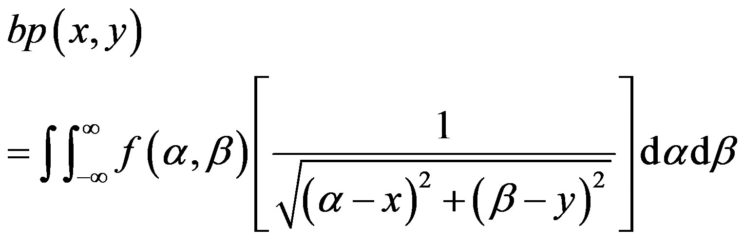 (15)
(15)
employing of convolution definition,
 (16)
(16)
Consequently,  , the reconstructed image by the back-projection method, is obtained by blurring
  by convoluting
 .
.
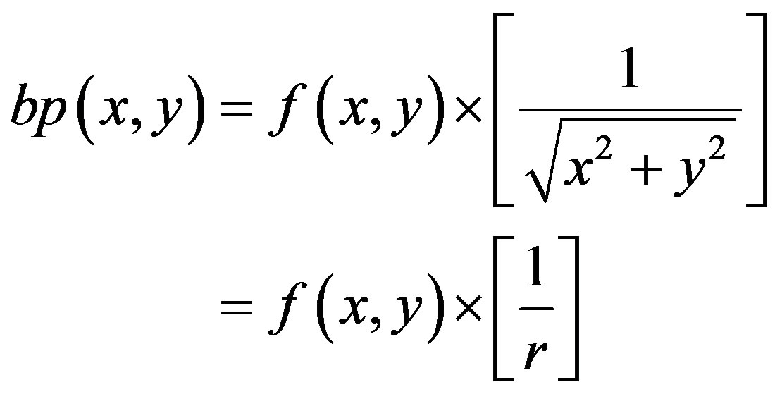
For a point source,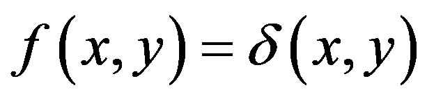 . Submitting this distribution function in Eq.15, we get
 (17)
(17)
Eq.15 indicates the intensity of the back-projection image rolls off slowly as  (see Figure 5).
3.3. The Back-Projection Filtering (BPF) Method
As said above, the reconstructed image by simple back-projection method is highly blurred and not the real reconstruction. However, the Fourier transformation Eq.16 yields×105
Figure 5. Surface plot of the backprojection image of a point source.
 (18(
(18(
 (19)
(19)
since,
 (20(
(20(
then,
 (21(
(21(
 (22)
(22)
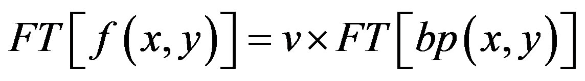
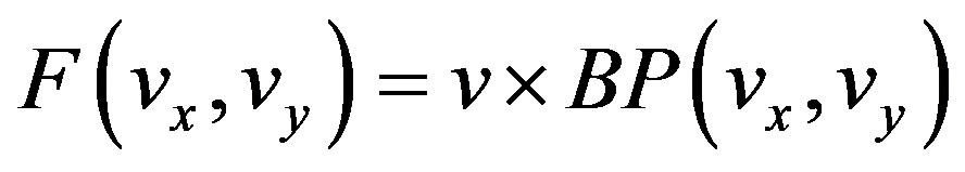
where  is the 2-D Fourier transform of the back-projected image and
  is the 2-D Fourier transform of the back-projection-filtered image. Eq.22 yields the Fourier transform of the original object
 . This deblurring is called inverse filtering, and this kind of the inverse operation of convolution is called deconvolution [5,6].
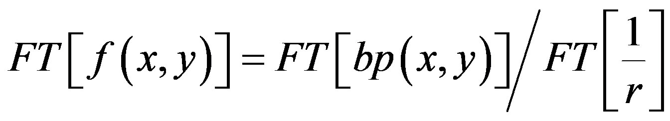
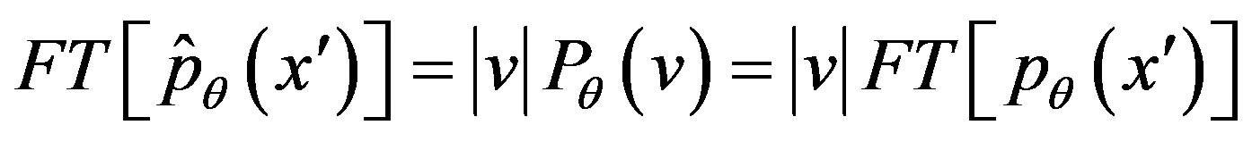
The final step is the inverse Fourier transform of  to obtain the image
 . According to convolution theorem, the product of the Fourier transforms of the two functions in frequency space equals to the convolution of two functions in spatial space, i.e.
 (23)
(23)
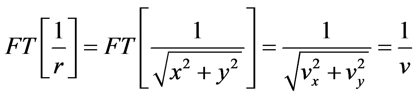
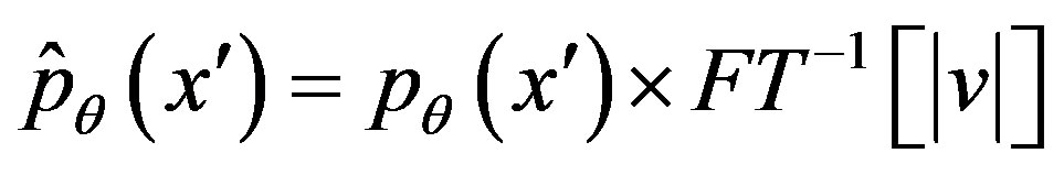
This is known as the back-projection filtering (BPF) image reconstruction method, where the projection data are first back-projected, filtered in Fourier space with the cone filter, and then inverse Fourier transformed. Alternatively, the filtering can be performed in image space via the convolution of  with
with  (see Figure 6). A disadvantage of this approach is that the function
  has a larger support than
 due to the convolution with the filter term, which results in gradually decaying values outside the support of
 . Thus, any numerical procedure must first compute
  using of a significantly larger image matrix size than is needed for the final result. This disadvantage can be avoided by interchanging the filtering and back-projection steps as discussed in next method.
3.4. The Filtered Back-Projection (FBP) Method
A practical reconstruction method is derived from the back-projection method using the projection theorem. Since  is obtained by the inverse Fourier transformation of
  [3,7],
 (24)
(24)
converting Eq.24 into the polar coordinate ,
,
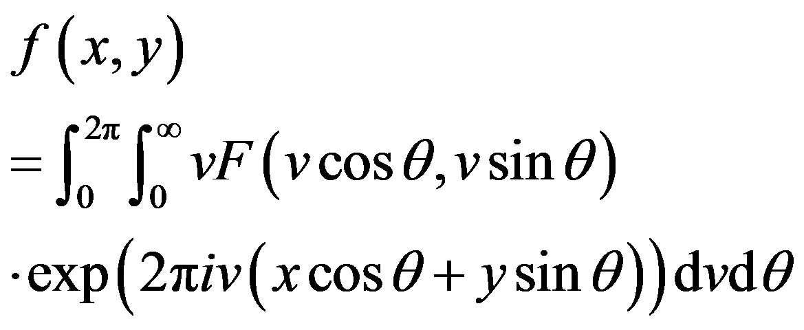 (25)
(25)
employing the Fourier slice theorem and separating the interval of integral (0, 2π) on θ as two subinterval (0, π) and (π, 2π), we get
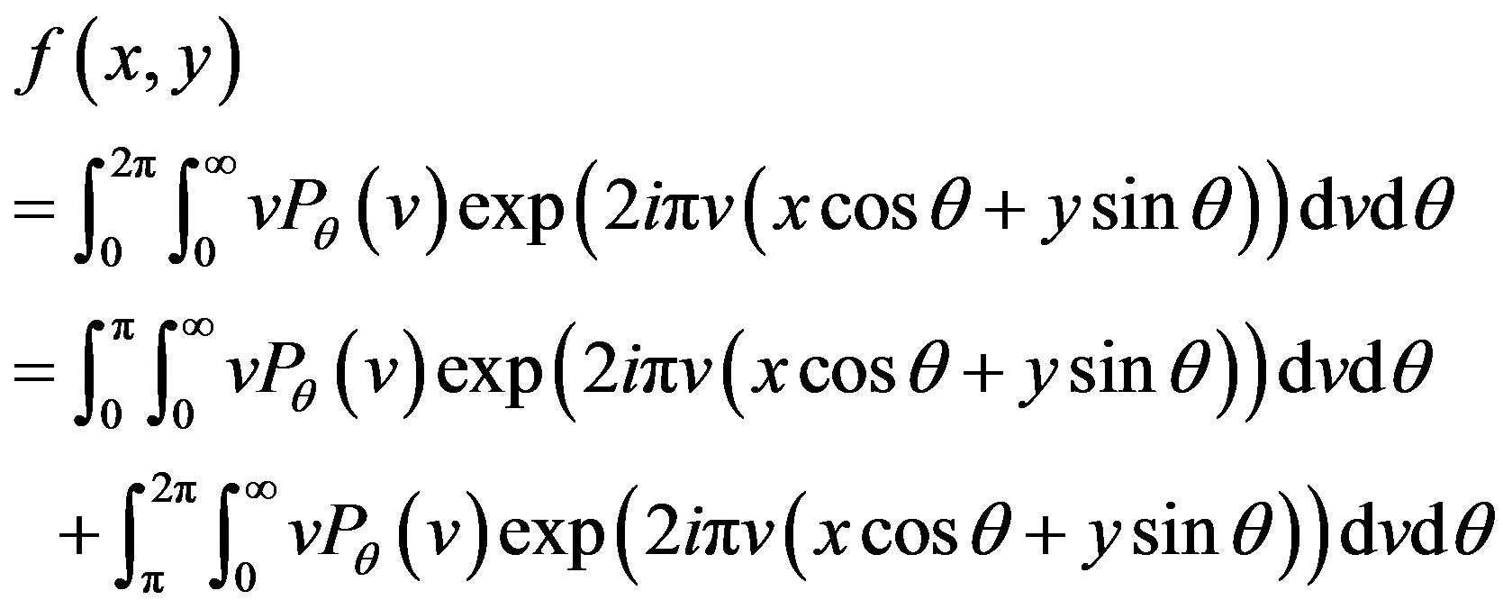 (26)
(26)
rewriting second term in summation and converting the subinterval (π, 2π) to (0, π), and the interval (0, ∞) to (–∞, 0), we get
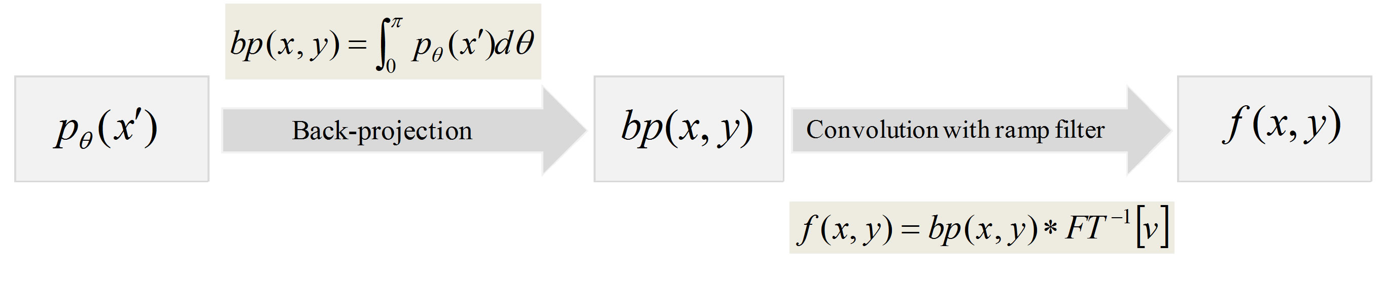
Figure 6. Flow of back-projection filtering (BPF) reconstruction method.
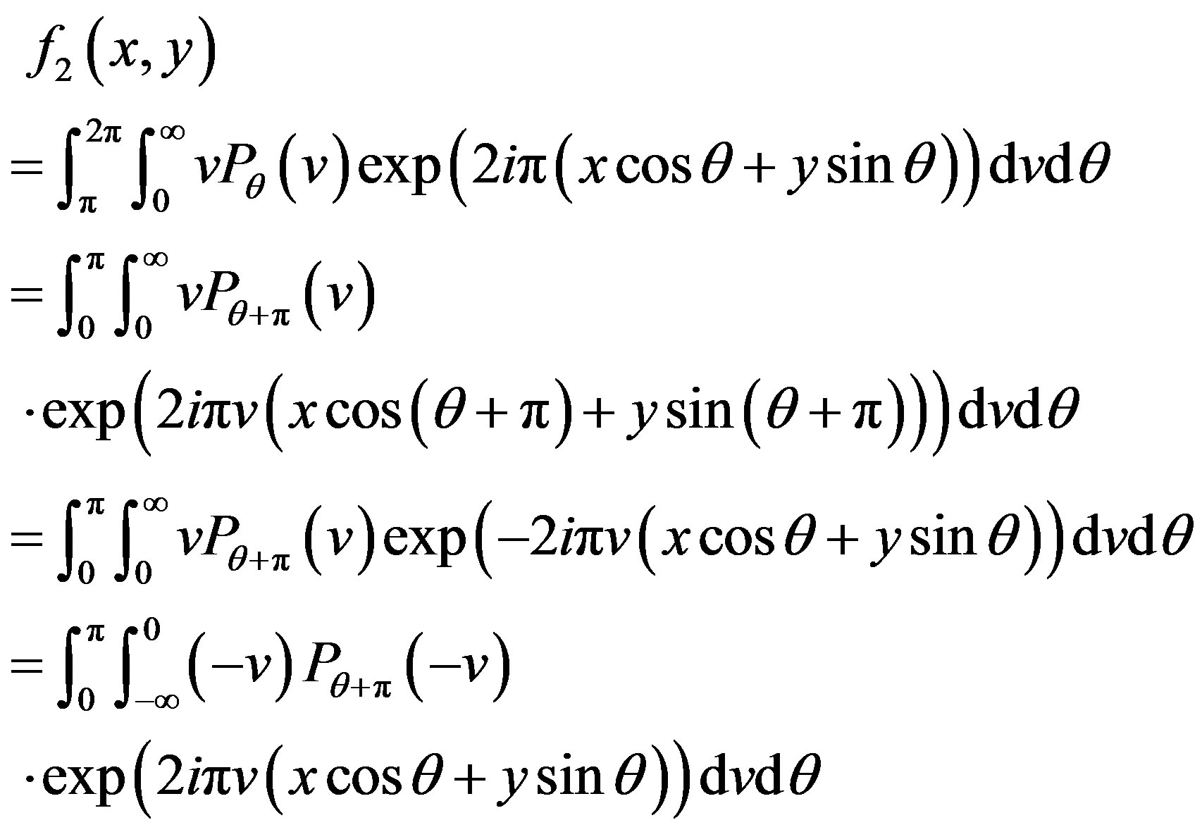 (27)
(27)
For parallel projection data, we clearly have
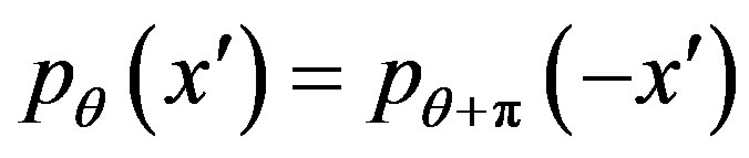 (28)
(28)
then, in frequency space,
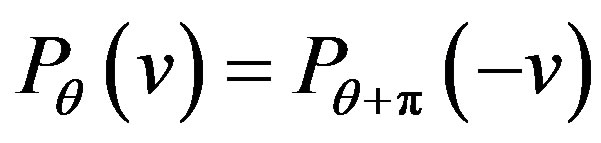 (29)
(29)
submitting Eq.29 into Eq.27 and rewriting Eq.26, we will get
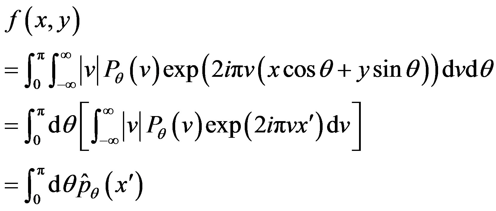 (30)
(30)
where
 (31)
(31)
Eq.30 is in the same form of the back-projection in Eq.9. The one-dimensional “ramp” filter,  , is a section through the rotationally symmetric two-dimensional cone filter (see Figure 7). Consequently, Eq.31 states that the original object
 is obtained by applying the filter that multiplies ramp filter to the Radon transforms and then performing the backprojection. This method is called filtered back-projection (FBP) method. This method performs the back-projection after applying the filter, contrarily to the back-projection with deconvolution, which is explained in the back-projection filtering method, which applies the filtering after the backprojection.
On the other hand, Since  is Fourier transform of
 , then
 (32)
(32)
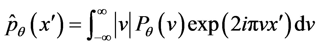
the Fourier transformation Eq.32 yields,
 (33)
(33)
This is a simple convolution and the Fourier transformation is not required. This method is called convolution back-projection method (see Figure 8).
4. DISCUSSION
Tomographic methods do not generate three dimensional images of an object directly. Instead sectional 2-D images are reconstructed from a set of projections. As the amount of data, or projections, is limited, there is not a unique solution. Due to the statistical nature of radioactive decay and detection process, the presence of noise in the acquired data is inevitable, so that an exact solution is not achievable. However, it is feasible to obtain a solution close to the given distribution, both in the visual and the quantitative aspects, so that a diagnostically reliable result is generally possible. We considered four analyticcal methods for reconstruction method here.
First method, Fourier transformation, although is theoretically the simplest of various reconstruction methods, it is practically not popular because obtaining projections for all θ is practically impossible; they are obtained at an interval of θ. The Fourier transformation of  is calculated practically by computers using the discrete Fourier transformation with sampled
 . Thus
  is obtained only at discrete points located radially on
  -plane. The discrete inverse Fourier transformation of
  requires
  at square lattice points. Since the radially located points and the lattice points are not generally synchronized, the values of
  at the lattice points have to be estimated from the values at the radially located points by some interpolation. The error by the interpolation in the frequency domain can yield an artifact, which is a noise not existing in the original image but caused by the processing, spread over the whole image. The artifact causes a severe misjudgment in image-aided medical diagnosis, since such diagnosis should find an object that should not be normally observed, for example a tumor.
In second method, back-projection (BP), the reconstructed image is blurred by convolution distribution function,  , with blurring factor,
 . Therefore, after back-projection, it is necessary to filter the oversampling in the Fourier space in order to have equal sampling throughout the Fourier space (see Figure 9).
For this reason, in third method, back-projection filtering (BPF), the Fourier transform of the back-projected image is filtered with a “cone” filter .
.
This cone filter accentuates values at the edge of the Fourier space and de-accentuates values at the center of Fourier space. However, this method has two problems:
1)  should be calculated within an area much broader than the support of
 , since the back-projection,
  , is spread by blurring
 .
.
2)  is positive at every
 since it is a distribution of absorbance. However, from Eq.22,
 when
when . It means that the DC component of
  is zero and negative values should appear in
 .This is a contradiction. The reason is that
  diverges at
  and no information on
  is obtained there. To avoid this advantage, in next method, back-projection and filtering steps is interchanged.
In fourth method, filtered back-projection, first projection data is filtered and then back-projected. This method does not require the inverse Fourier transformation of the spread blurred image, since the Fourier transformation is applied to the projections only. Although this method requires an interpolation between the polar coordinate to the Cartesian coordinate similarly to the Fourier transformation method, no artifact spread over the whole real domain is occurred, since this method carries out the interpolation in the real domain contrarily to the Fourier transformation method. Since the filtering can be applied for each θ independently, the filtering for a θ can be applied parallelly before the capture of projection at another θ is completed.
In general, the most well known of these methods is the filtered back-projection (FBP), based on the Central Slice Theorem and easy to be implemented. On the other hand, it does not take into account any of the factors that
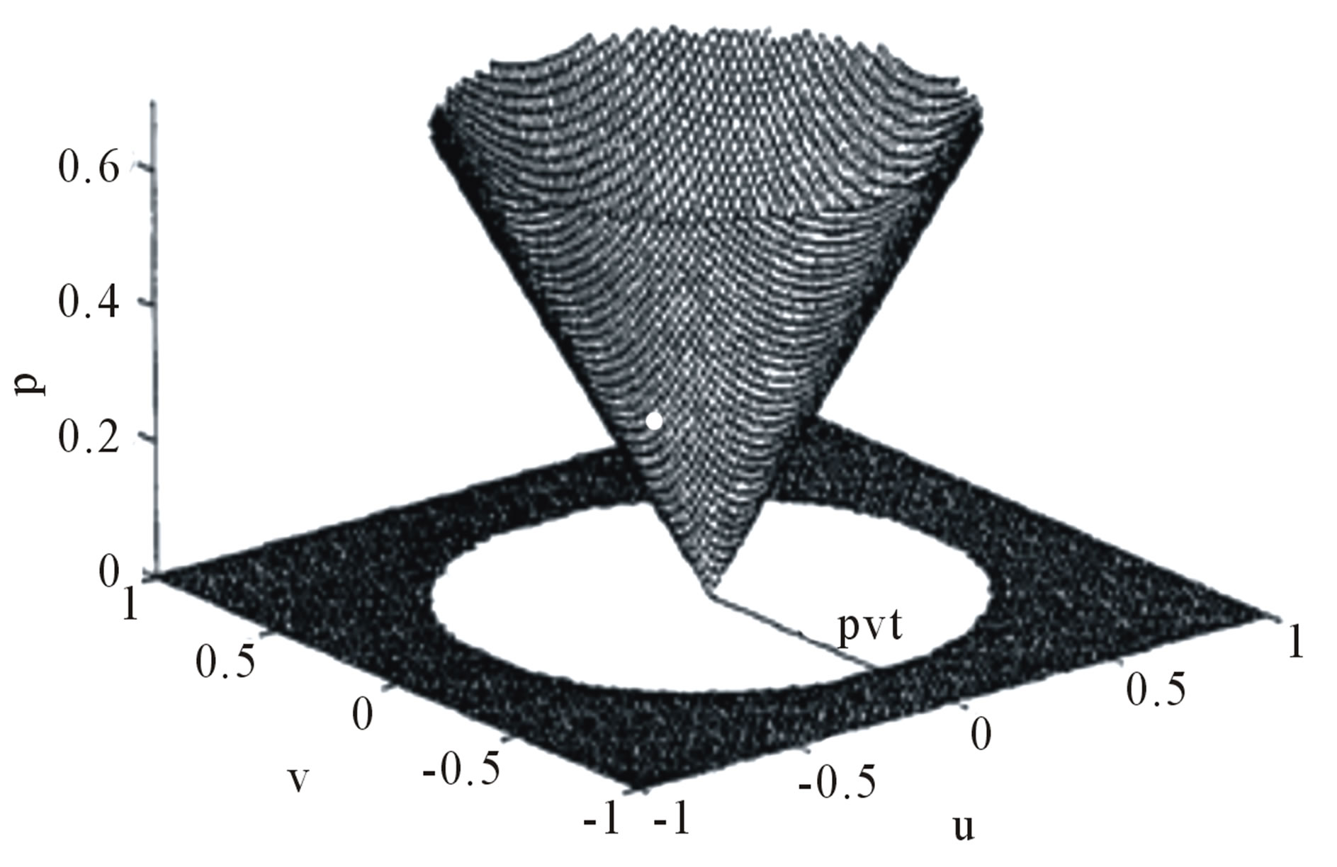
Figure 7. Illustration of cone ramp filter.
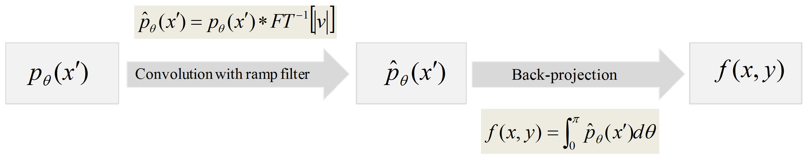
Figure 8. Flow of filtered back-projection (FBP) method.
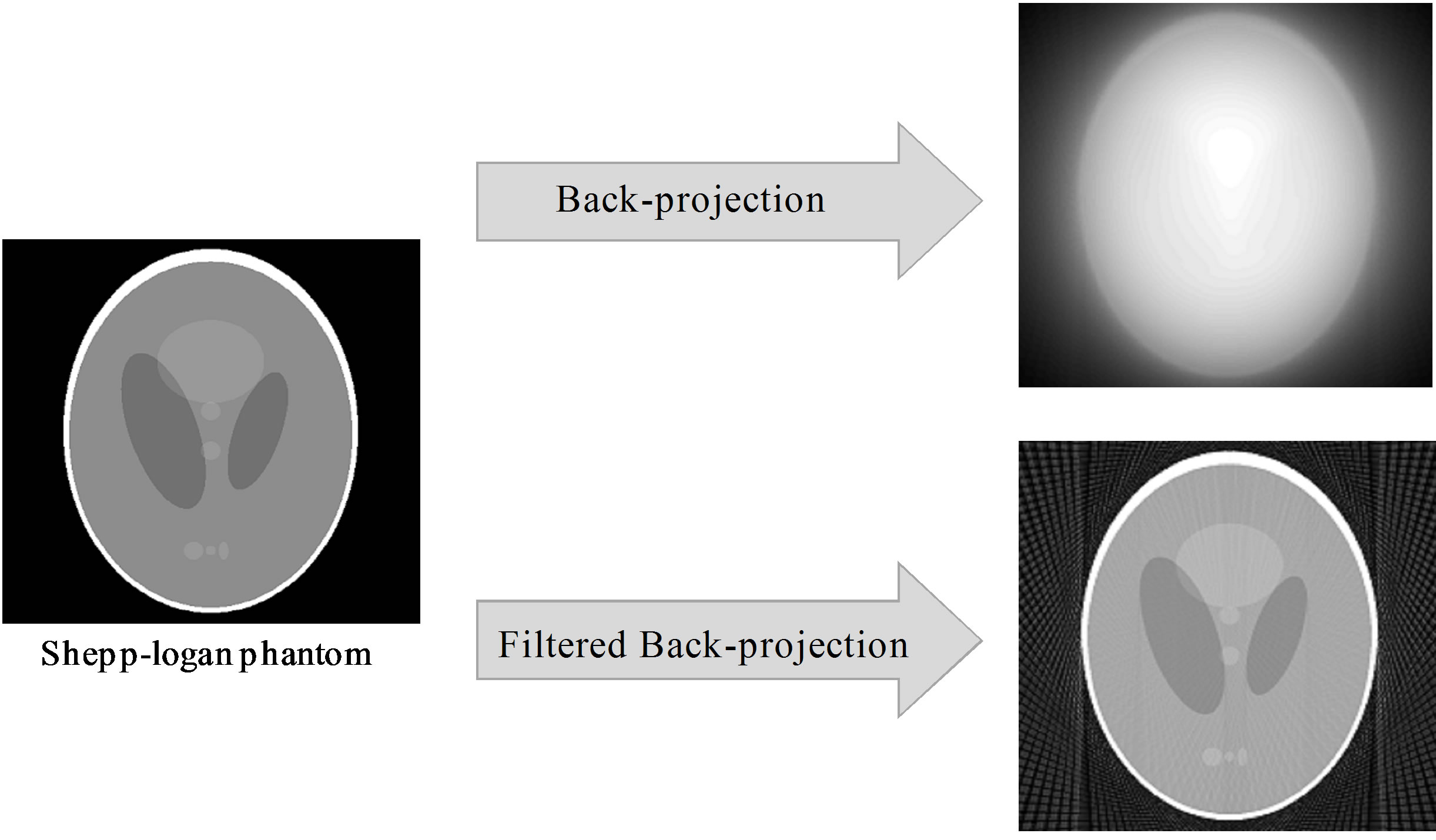
Figure 9. Comparative displaying of BP and FBP methods.
were mentioned before and considers the data noiseless. Therefore, it is necessary to perform radiation interactions correction either before or after the reconstruction. In general, FBP is available in all commercial nuclear medicine imaging systems and the resulting images are adequate for the majority of routine clinical problems.
REFERENCES
- Defrise, M. and Kinahan, P.E. (1998) Data acquisition and image reconstruction for 3D PET. In: Townsend, D.W. and Bendriem, B., Eds., The Theory and Practice of 3D PET, Developments in Nuclear Medicine, Kluwer Academic Publishers, Dordrecht, 32, 11-54.
- Jain A.K. (1988) Fundamentals of digital image processing. Prentice Hall, Upper Saddle River.
- Herman, G.T. (1980) Image reconstruction from projections. Academic Press, New York.
- Jähne, B. (1991) Digital image processing: Concepts, algorithms and scientific applications. Springer-Verlag, Berlin.
- Kak, A.C. (1984) Image reconstruction from projections. In: Ekstrom, M.P., Image Processing Techniques, Computational Techniques, Academic Press, Orlando, 2, 111- 169.
- Bruyant, P.P. (2002) Analytic and iterative reconstruction algorithms in SPECT. Journal of Nuclear Medicine, 43, 1343-1358.
- Kinahan, P.E. and Rogers, J.G. (1989) Analytic 3D image reconstruction using all detected events. IEEE Transactions on Medical Imaging, 36, 964-968.