Intelligent Control and Automation
Vol. 3 No. 4 (2012) , Article ID: 24892 , 6 pages DOI:10.4236/ica.2012.34045
A Reward Functional to Solve the Replacement Problem
Academic Area of Engineering, Autonomous University of Hidalgo, Pachuca, México
Email: evah@uaeh.edu.mx
Received May 5, 2012; revised August 22, 2012; accepted August 30, 2012
Keywords: Markov Chains; Dynamic Programming; Replacement Problem
ABSTRACT
The replacement problem can be modeled as a finite, irreducible, homogeneous Markov Chain. In our proposal the problem was modeled using a Markov decision process and then, the instance was optimized using dynamic programming. We proposed a new functional that includes a reward functional, that can be more helpful in processing industries because it considerate instances like incomes, maintenance costs, fixed costs to replace equipment, purchase price and salvage values; and this functional can be solved with dynamic programming and used to make effective decisions. Two theorems are proved related with this new functional. A numerical example is presented in order to demonstrate the utility of this proposal.
1. Introduction
The machine replacement problem has been studied by a lot of researchers and is also an important topic in operations research, industrial engineering and management science. Items which are under constant usage, need replacement at an appropriate time as the efficiency of the operating system that uses such items suffer a lot. In this proposal we include a reward functional, that is more helpful in processing industries because it considerate instances like incomes, maintenance costs, fixed costs to replace equipment, purchase price and salvage values; and this functional can be solved with dynamic programming and used to make effective decisions.
In the real-world the equipment replacement problem involves the selection of two or more machines of one or more types from a set of several possible alternative machines with different capacities, cost of purchase and operation to produce efficiently. When the problem involves a single machine, it is common to find two welldefined forms of this; the quantity-based replacement, and the time-based replacement. In the quantity-based replacement model, a machine is replaced when an accumulated product of size q is produced. In this model, one has to determine the optimal production size q. While in a time-based replacement model, a machine is replaced in every period of T with a profit maximizing.
When the problem involves two or more machines this problem is named the parallel machine replacement problem, and the time-based replacement model consists of finding a minimum cost replacement policy for a finite population of economically interdependent machines.
A replacement policy is a specification of “keep” or “replace” actions, one for each period. Two simple examples are the policy of replacing the equipment every time period and the policy of keeping the first machine until the end of a period N. An optimal policy is a policy that achieves the smallest total net cost of ownership over the entire planning horizon and it has the property that whatever the initial state and initial decision are, the remaining decisions must constitute an optimal policy with regard the state resulting from the first decision. In practice, the replacement problem can be easily addressed using dynamic programming and Markov decision processes.
The dynamic programming uses the following idea: The system is observed over a finite or infinite horizon split up into periods or stages. At each stage the system is observed and a decision or action concerning the system has to be made. The decision influences (deterministically or o stochastically) the state to be observed at the next stage, and depending on the state and the decision made, an immediate reward is gained. The expected total rewards from the present stage and the one of the following state is expressed by the functional equation. Optimal decisions depending on stage and state are determined backwards step by step as those maximizing the right hand side of the functional equation [1]. Howard [2] combines the dynamic programming technique with the mathematically well established notion of a Markov chain, creating the new concept called the Markov Decision processes and developing the solution of infinite stage problems. The policy iteration method was created as an alternative to the stepwise backward contraction methods. The policy iteration was a result of the application of the Markov chain environment and it was an important contribution to the development of optimization techniques [1].
In this document, a stochastic machine replacement model is considered. The system consists of a single machine and this is assumed to operate continuously and efficiently over N periods. In each period, the quality of the machine deteriorates due to its use, and therefore, it can be in any of the N states, denoted 1, 2, ···, N. In our proposal we modeled the problem using a Markov decision process and then, the instance is optimized using dynamic programming. We propose a new functional that includes a reward function, also helpful information as incomes, maintenance costs, fixed costs to replace equipment, purchase price and salvage values. Two theorems are proved related with this new functional.
In this proposal is assumed that for each new machine it state can become worse or may stay unchanged, and that the transition probabilities pij are known, where
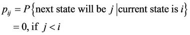
also be assumed that the state of the machine is known at the start of each period, and we must choose one of the following two options: a) Let the machine operate one more period in the state it currently is, b) Replace the machine by a new one, where every new machines for replacement are assumed to be identical.
2. Literature Review
There are several theoretical models for determining the optimal replacement policy. The basic model considers maintenance cost and resale value, which have their standard behavior as per the same cost during earlier period and also partly having an exponential grown pattern as per passage of time. Similarly the scrap value for the item under usage can be considered to have a similar type of recurrent behavior. In relation to stochastic models the available literature on discrete time maintenance models predominantly treats an equipment deterioration process as a Markov chain.
Sernik and Marcus [3], obtained the optimal policy and its associated cost for the two-dimensional Markov replacement problem with partial observations. They demonstrated that in the infinite horizon, the optimal discounted cost function is piecewise linear, and also provide formulas for computing the cost and the policy. In [4], the authors assume that the deterioration of the machine is not a discrete process but it can be modeled as a continuous time Markov process, therefore, the only way to improve the quality is by replacing the machine by one new. They derive some stability conditions of the system under a simple class of real-time scheduling/replacement policy.
Some models are approached to evaluate the inspecttion intervals for a phased deterioration monitored complex components in a system with severe down time costs using a Markov model (see [5], for example).
In [6], the problem is approached from the perspective of the reliability engineering developing replacement strategies based on predictive maintenance. Moreover in [7] the authors formulated a stochastic version of the parallel machine replacement problem. They analyzed the structure of optimal policies under general classes of replacement cost functions.
Another important approach that has received the problem is the geometric programming [8]. In its proposal, the author discusses the application of this technique to solving replacement problem with an infinite horizon and under certain circumstances he obtains a closed-form solution to the optimization problem.
A treatment to the problem when there are budget constraints can be found in [9]. In their work, the authors propose a dual heuristic for dealing with large, realistically sized problems through the initial relaxation of budget constraints.
Compared with simulation techniques, Dohi et al. [10], propose a technique based on obtaining the first two moments of the discounted cost distribution, and then, they approximate the underlying distribution function by three theoretical distributions using Monte Carlo simulation.
The most important pioneers in applying dynamic programming models in replacement problems are: Bellman [11], White [12], Davidson [13], Walker [14] and Bertsekas [15]. Recently the Markov decision process has been applied successfully to the animal replacement problem as a productive unit (see [16-18], for example).
Although the modeling and optimization of the replacement problem using Markov decision processes is a topic widely known [19]. However, there is a significant amount about the theory of stochastic perturbation matrices (see [20-23], and references therein). Considering all the references, the problem is presented in the next section.
3. Problem Formulation
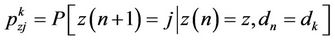
We start by defining a discrete-time Markov decision process with a finite state space Z states z1, z2, ···, zz where, in each stage s = 1, 2, ··· the analyst should made a decision d between ξ possible. Denote by z(n) = z and d(n) = di the state and the decision made in stage n respectively, then, the system moves at the next stage n + 1 in to the next state j with a know probability given by
 (1)
(1)
When the transition occurs, it is followed by the reward  and the payoff is given by
at the state z after the decision dk is made.
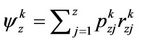
For every policy  the corresponding Markov chain is ergodic, then the steady state probabilities of this chain are given by
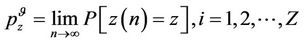
and the problem is to find a policy  for which the expected payoff is
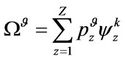 (2)
(2)
is maximum. In this system, the time interval between two transitions is called a stage.
An optimal policy is defined as a policy that maximizes (or minimizes) some predefined objective function. The optimization technique (i.e. the method to obtain an optimal policy) depends on the form of the objective function and it can result in different alternative objective function. The choice of criterion depends on whether the planning horizon is finite or infinite [1].
In our proposal we consider a single machine and regular times intervals whether it should be kept for an additional period or it should be replaced by a new. By the above, the state space is defined by 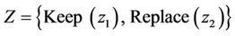 and having observed the state, action should be taken concerning the machine about to keep it for at least an additional stage or to replace it at the end of the stage.
The economic returns from the system will depend on its evolution and whether the machine is kept or replaced, in this proposal this is represented by a reward depending on state and action specified in advance. If the action replace is taken, we assume that the replacement takes place at the end of the stage at a known cost, the planning horizon is unknown and it is regarded infinite, also, all the stages are of equal length.
The optimal criterion used in this document is the maximization of the expected average reward per unit of time given by
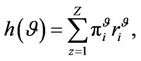 (3)
(3)
where  is the limiting state probability under the policy.
Traditionally dynamic programming is recognized as a method to solve complex problems based on their decomposition in simpler models. By the way of operate, this technique is applied in cases where problems have optimal substructure.
The basic model contains two main elements: a) a discrete dynamical system that evolves over time, b) a cost function that is additive over time [15]. The system evolves under the influence of pro decisions expressed through state variables and has the form
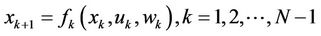 (4)
(4)
where k is the discretized time index.
xk is the state of the system and keep the past information that is relevant to future optimization.
uk is the decision variable that must be choose in time k.
wk is the decision random parameter (or noise).
N is the planning horizon.
And fk is a function that describes the system. The cost function is additive because the cost of time k,  is accumulated over the time. The total cost is
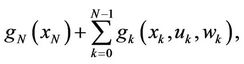 (5)
(5)
where  is the final cost in the end of the process. Although, because the presence of wk, this cost is generally a random variable and don’t have any sense to optimize it as a punctual value, in this case, the expected cost is used
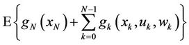 (6)
(6)
the expected value is applied over the join distribution of the random variables involved in the process. The optimization is over the decision variables u0, u1, ···, uN–1. In turn, the random variables uk are selected with updated information on the current state variable xk either exact or approximate values. This section proposes to use the methodology of dynamic programming to solve replacement problem using a reward function constructed from the functions of cost and incomes.
4. A Functional Associated with the Reward
In this section we presented the replacement problem as a dynamic system that evolves certain laws that are included in the transition probability matrices. In this case, the cost function of the system in the state i is g(i) and satisfies that
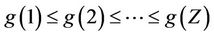 (7)
(7)
this means that the cost is state i is less than the cost in the state i + 1 and the state 1 corresponds to best equipment condition, Z represents all the states in the system. Generally, between each operation period the equipment may worsen or remain unchanged. Then, for the stochastic case the transition probabilities are
 (8)
(8)
It is suppose that in the beginning of the next period, the state of the equipment is known and the following two decisions must be chosen: a) maintain the operation of the equipment for a next period and b) repair the equipment to take the state 1 at a cost R. Another important hypothesis is that after the equipment is repaired, the state 1 is guaranteed for at least one period, and in the following periods, the equipment may be worsen according to the transition probabilities pij.
Considering the above, the problem is to determine the deterioration level (state) where the lower cost of repairing the machine is obtained, therefore, the best benefits in relation to the cost will be obtained in the future.
Although the ease of dynamic programming to represent the states is an advantage, it is also true that the computational complexity increases when more possibilities of the system are considerate. Our approach consists of a reward functional that includes the expenses and the benefits proportioned by the equipment with two states (keep and replace), although more than two states could be considerate.
Formally, the reward function is
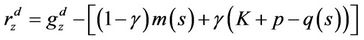 (9)
(9)
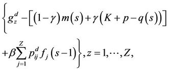
where  represent the incomes obtained when the process is the state z and the decision d is taken. Similarly, the expression
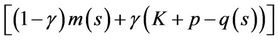 (10)
(10)
represents the outgoings made in the maintenance or the replacement of the equipment, when the equipment works s stages before its replacement. Here, m(s) represents the maintenance cost when the equipment is in the stage s, K are the fixed costs to replace the equipment, p is the purchase price of a new equipment and q(s) is the rescue value when the equipment is in the stage s. The constant γ is
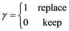 (11)
(11)
Suppose now that the costs are bounded and ξ is such that
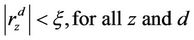
Then, using the Equation (9) the next functional is proposed
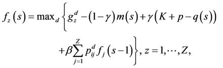 (12)
(12)
to evaluate the expected reward of the process in all the stages. If can be proved (see [15],) that in this approach the discount factor β, 0 < β < 1, is used in order to ensure that the reward obtained in the future will be less than the reward obtained in the present. So, considerating the  policy
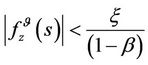 (13)
(13)
Let
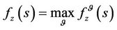 (14)
(14)
here, it is said that a policy is β-optimal.
Then, a policy is β-optimal is the reward β-discounted is maximum for every initial value. This proposal could be formalized in the following theorems Theorem 4.1: The functional

satisfies the optimal value of .
.
Proof: The proof is trivial. This approach is a variant of the optimality equation proposed and demonstrated by Ross [24], where the functional is written through the reward function as
 .
.
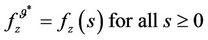
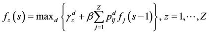
Theorem 4.2: Let  a stationary policy, so if the process is in the state z, the decision d is chosen in order to maximize the function
So 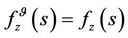 for all s > 0, then f is a function β- optimal.
Proof: Rewriting the functional of the Equation (11), again we have a variant of the optimality equation of Ross [24], that is demonstrated in this reference.
5. Numerical Example
Consider a variation of the example reported in [2], the incomes  are in Table 1.
The Table 2 shows the transition probabilities reported in [1], which represented a Markovian decision process with d = {K, R}.
The maintenance costs are variable in every stage increasing at a rate of 1%, the maintenance cost in the stage s = 1 is m(1) = 10,000. The rescue value also changes in every stage decreasing at a rate of 10%, for the first stage is q(1) = 2000. In Table 3 are some maintenance costs and rescue values for the first 40 stages.
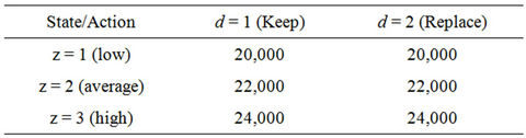
Table 1. Incomes, .
.
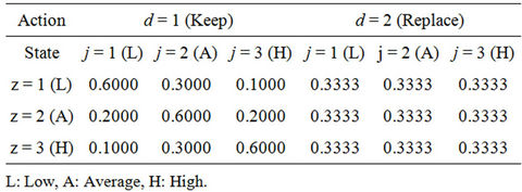
Table 2. Transition probabilities, .
.
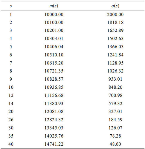
Table 3. Maintenance costs, m(s) and rescue values.
Equipment is K = 3000, and the purchase price of a new equipment is p = 10,000. A discounted factor of β = 0.9 and a planning horizon of s = 40 are considered.
In the Table 4 are showed the iterations from the first s = 40 stages. Note that from s = 1 to s = 25, the result is replace in the state z = 1 and keep in the states z = 2, 3. From s = 26 to s = 33, the result is replace in the states z = 1, 2 and keep in the state z = 3. From s = 34, the decision is replace in the three states. These results are obtained because the maintenance costs are increasing and the rescue values are decreasing from one stage to another.
6. Conclusions
For replacement problems with finite planning horizon, dynamic programming has been the most widely used technique; this is because using this technique because it is possible to deduce the optimal solution naturally through functional forms.
In our approach we explore the replacement problem solved by dynamic programming and we propose a new functional that includes a reward function, also helpful information as incomes, maintenance costs, fixed costs to replace equipment, purchase price and salvage values. Two theorems are proved related with this new func-
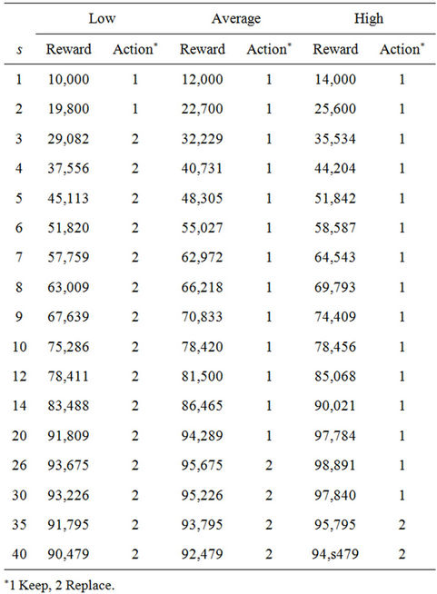
Table 4. Numerical results.
tional. Future work could be to include more decisions (not only keep and replace), this decisions complicate the solution but is more similar to real life. Other contribution could be increase the number of equipments, the incomes and costs related to the replacement problem.
This model has been developed without considering a specific kind of industry, but can be used in the processing industry, now we are working to validate the model in some processing industries in our region.
REFERENCES
- A. Kristensen, “Textbook Notes of Herd Management: Dynamic Programming and Markov Process,” Dina Notat, 1996. http://www.husdyr.kvl.dk/ark/pdf/notat49.pdf
- R. A. Howard, “Dynamic Programming and Markov Processes,” The MIT Press, Cambridge, 1960.
- E. L. Sernik and S. Marcus, “Optimal Cost and Policy for Markovian Replacement Problem,” Journal of Optimization Theory and Applications, Vol. 71, No. 1, 1991, pp. 105-126. doi:10.1007/BF00940042
- S. P. Sethi, G. Sorger and X. Zhou, “Stability of RealTime Lot Scheduling and Machine Replacement Policies with Quality Levels,” IEEE Transactions on Automatic Control, Vol. 45, No. 11, 2000, pp. 2193-2196. doi:10.1109/9.887687
- J. D. Sherwin and B. Al-Najjar, “Practical Models for Conditions-Based Monitoring Inspection Intervals,” Journal of Quality in Maintenance Engineering, Vol. 5, No. 3, 1999, pp. 203-209. doi:10.1108/13552519910282665
- E. Lewis, “Introduction to Reliability Theory,” Wiley, Singapore City, 1987.
- S. Childress and P. Durango-Cohen, “On Parallel Machine Replacement Problems with General Replacement Cost Functions and Stochastic Deterioration,” Naval Research Logistics, Vol. 52, No. 5, 1999, pp. 402-419.
- T. Cheng, “Optimal Replacement of Ageing Equipment Using Geometric Programming,” International Journal of Production Research, Vol. 30, No. 9, 1999, pp. 2151- 2158. doi:10.1080/00207549208948142
- N. Karabakal, C. Bean and J. Lohman, “Solving Large Replacement Problems with Budget Constraints,” The Engineering Economist, Vol. 4, No. 5, 2000, pp. 290-308. doi:10.1080/00137910008967554
- T. Dohi, et al., “A Simulation Study on the Discounted Cost Distribution under Age Replacement Policy,” Industrial Engineering and Management Sciences, Vol. 3, No. 2, 2004, pp. 134-139.
- R. Bellman, “Equipment Replacement Policy,” Journal of Society for Industrial and Applied Mathematics, Vol. 3, No. 3, 1955, pp. 133-136.
- D. White, “Dynamic Programming,” Holden Day, San Francisco, 1969.
- D. Davidson, “An Overhaul Policy for Deteriorating Equipment,” In: A. Jardine, Ed., Operational Research in Maintenance, Manchester University Press, New York, 1970, pp. 1-24.
- J. Walker, “Graphical Analysis for Machine Replacement,” International Journal of Operations and Production Management, Vol. 14, No. 10, 1992, pp. 54-63. doi:10.1108/01443579410067252
- D. Bertsekas, “Dynamic Programming and Optimal Control,” Athena Scientific, Belmont, 2000.
- L. Plá, C. Pomar and J. Pomar, “A Markow Sow Model Representing the Productive Lifespan of Herd Sows,” Agricultural Systems, Vol. 76, No. 1, 2004, pp. 253-272.
- L. Nielsen and A. Kristensen, “Finding the K Best Policies in a Finite-Horizon Markov Decision Process,” European Journal of Operation Research, Vol. 175, No. 2, 2006 pp. 1164-1179. doi:10.1016/j.ejor.2005.06.011
- L. Nielsen, et al., “Optimal Replacement Policies for Dairy Cows Based on Daily Yield Measurements,” Journal of Dairy Science, Vol. 93, No. 1, 2009, pp. 75-92. doi:10.3168/jds.2009-2209
- F. Hillier and G. Lieberman, “Introduction to Operations Research,” Mc. Graw Hill Companies, Boston, 2002.
- P. Schrijner and E. Doorn, “The Deviation Matrix of a Continuous-Time Markov Chain,” Probability in the Engineering and Informational Science, Vol. 16, No. 3, 2009, pp. 351-366.
- C. Meyer, “Sensitivity of the Stationary Distribution of a Markov Chain,” SIAM Journal of Matrix Applications, Vol. 15, No. 3, 1994, pp. 715-728. doi:10.1137/S0895479892228900
- M. Abbad, J. Filar and T. R. Bielecki, “Algorithms for Singularly Perturbed Markov Chain,” Proceedings of the 29th IEEE Conference, Honolulu, 5-7 December 1990, pp. 1402-1407.
- E. Feinberg, “Constrained Discounted Decision Processes and Hamiltonian Cycles,” Mathematical Operational Research, Vol. 25, No. 1, 2000, pp. 130-140. doi:10.1287/moor.25.1.130.15210
- S. Ross, “Applied Probability Models with Optimization Applications,” Holden Day, San Francisco, 1992.