Journal of Modern Physics
Vol.4 No.6(2013), Article ID:33086,16 pages DOI:10.4236/jmp.2013.46109
Absolute Maximum Proper Time to an Initial Event, the Curvature of Its Gradient along Conflict Strings and Matter
R&D Algorithms Department, ANB/ANT—Applied Neural Biometrics/Technology, Netanya, Israel
Email: eytan_il@netvision.net.il, eytansuchard@gmail.com
Copyright © 2013 Eytan H. Suchard. This is an open access article distributed under the Creative Commons Attribution License, which permits unrestricted use, distribution, and reproduction in any medium, provided the original work is properly cited.
Received January 22, 2013; revised February 28, 2013; accepted April 1, 2013
Keywords: Foliation; Field Curvature; General Relativity; Accelerated Cosmic Expansion; Quantum Gravity; Dark Matter; Chameleon Scalar Field
ABSTRACT
Einstein equation of gravity has on one side the momentum energy density tensor and on the other, Einstein tensor which is derived from Ricci curvature tensor. A better theory of gravity will have both sides geometric. One way to achieve this goal is to develop a new measure of time that will be independent of the choice of coordinates. One natural nominee for such time is the upper limit of measurable time form an event back to the big bang singularity. This limit should exist despite the singularity, otherwise the cosmos age would be unbounded. By this, the author constructs a scalar field of time. Time, however, is measured by material clocks. What is the maximal time that can be measured by a small microscopic clock when our curve starts at near the “big bang” event and ends at an event within the nucleus of an atom? Will our tiny clock move along geodesic curves or will it move in a non geodesic curve within matter? It is almost paradoxical that a test particle in General Relativity will always move along geodesic curves but the motion of matter within the particle may not be geodesic at all. For example, the ground of the Earth does not move at geodesic velocity. Where there is no matter, we choose a curve from near “big bang” to an event such that the time measured is maximal. Without assuming force fields, the gravitational field which causes that two or more such curves intersect at events, would cause discontinuity of the gradient of the upper limit of measurable time scalar field. The discontinuity can be avoided only if we give up on measurement along geodesic curves where there is matter. In other words, our tiny test particle clock will experience force when it travels within matter or near matter.
1. Introduction: Square Curvature in Positive Definite Metric Spaces
A) Ideas
• If spacetime is homotopic to a single starting event, say “big bang” then maximal proper time curves can be drawn back from any event, to a limit that converges at the big bang singularity. Along these curves we can imagine a tiny clock that travels and measures time. This time is considered as a scalar field. Clock tick is different under local space location due to gravity. The scalar field therefore, has a significant gradient by space. Where there is matter, however, a tiny particle-like clock will never move along geodesic curves because as we shall see, it would lead to discontinuities in the gradient of our scalar field of upper limit of measurable time. The expected subatomic force deviates from any non-Newtonian model in that the force is trajectory and speed dependent because it means that a particle that moves along a trajectory and indeed measures the upper limit can’t be geodesic near matter.
• The laws of Nature will never directly involve any absolute time. Instead, we will be coerced to define them by using the gradient of such time, which is indeed local. This point is crucial to the understanding of this paper! Also crucial is to understand the time discussed in this paper is well defined as an upper limit on measurable proper time.
• A nice, though less important issue, is that deconstructing space time into 3 + 1 dimensions require local time orthogonality unlike in Kerr solution. This idea will also be addressed though it is a bit speculative.
2. Classical Matter: The Gradient Need Not to Be Parallel to any Geodesic Curve, Resolving Singularities
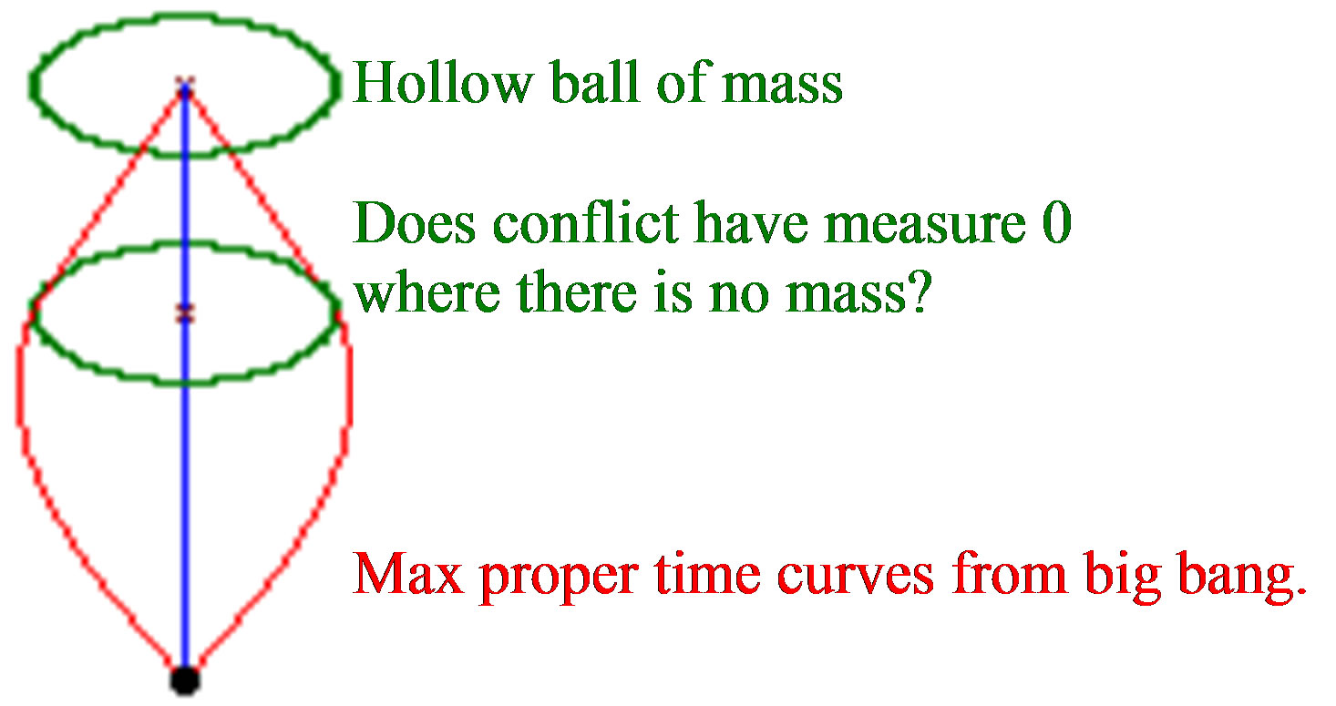
Our strategy now will be to see what would happen to the gradient of the upper limit of measurable time from any event backwards, if no forces act on our test-clock-particles. Then to show that forces are indeed required for avoiding singularities at curve intersections. The direction in space time of the particles measuring the maximum proper time forms a geodesic curve but near matter, without the existence of forces, not necessarily the gradient of the field would be parallel to a geodesic curve because: 1) more than one curve could reach the same event; 2) at that event near matter, even known forces would cause any test particle clock to move along non geodesic curves; and 3) one idea, even without explicitly assuming forces near matter, is that in a quantum model the intersection of such curves does manifest singularity of the gradient but by coupling by multiplication of the time field and a wave function of the entire system of particles, the 4-loaction of the singularity can be blurred by uncertainty. Whichever model we choose 2 or 3, a real world clock will not move along geodesic curves within matter, otherwise its measurement will result in discontinuities or singularities of the gradient of our upper limit on measurable time. The idea of such particle clocks is not quite new [1] and is important in order to have physical meaning. A good example of discontinuity is the center and edge of a hollowed ball of mass, see Figure 1(a). Due to General Relativity, the clock ticks in the gravitational field of the ball are slower than far from the ball. As a result, max proper time geodesic curves from say “big bang” event, must come from outside the ball into the ball. The time at the center of the ball is also a geodesic curve but it is in the time direction in Schwarzschild coordinates due to symmetry. The vector field of the lines is therefore discontinuous and we have a non-zero Euler number [2] of the gradient field. As was already mentioned, one way to resolve such singularities is that our particle clock will experience force. Spacetime in a hollow ball of mass is conic i.e. the metric coefficient  of the radius difference
  is greater than 1, and is thus flat but with a zero measure singularity of the Gaussian curvature at the center which is the tip of 4 dimensional cone. In any case such force has to be negligible though it should exist and should disallow geodesic movement in the sub atomic scale that will otherwise manifest the gradient singularity.
If we consider the ideas of Quantum Gravity, “conflict” events where curves intersect do not have zero measure. But as was already mentioned, even without quantum gravity it is not difficult to imagine that such singularities can be avoided in the sub-atomic level by force that prevents any microscopic real world clock from moving along geodesic curves. Our field of time then sets an upper limit to measurable time by any such tiny clock particle. The conflict is apparent also on the edges of the ball because matter is granular, that is to say that the mass is not evenly distributed. Particles measuring absolute maximum proper time from near “big bang” along curves that enter the ball, must pass through the walls of the ball or hyper-cylinder in 4 dimensions. Therefore, gravitational lenses are formed and events in the hollowed part of the ball are accessible by more than one curve as depicted by Figure 1(b). These singularities can be resolved too if any real world particle-like clock will not move along geodesic curves in the microscopic vicinity of matter, e.g. due to Casimir/Casimir Lifshitz [3].
Again, the newly presented type of gradient conflicts (also caused by absolute maximum proper time intersections) events can be avoided by either providing that the matter’s time and location are uncertain or by force exerted on the test-clock-particles. If we say that matter is measured by such conflicts/intersections, then the fact we also have a microscopic, though negligible geodesic conflict in the center of the ball, attests to the existence of a new type of mass, we can call “Secondary Dark Matter”, that mass is not additional to the mass of the ball but simply means that some force field which relates to matter can weakly extend beyond the microscopic scale. In
 (a)
(a) (b)
(b)
Figure 1. (a) The line of the max proper time field from “big bang” is discontinuous in the middle of a hollowed ball of mass and therefore a real world clock will not move along geodesic curves at such points, no matter how negligible is such an effect; (b) On the edges, gravitational lenses due to granularity cause geodesic conflicts. The particles form an obstacle that is bypassed by the entering curves.
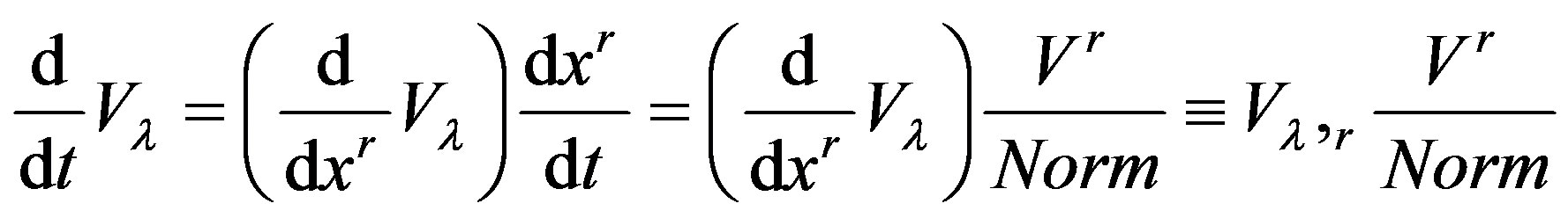
big words, the theory that is behind this paper says that indeed, laws of physics are local but the entire geometric context have influence on a new effect we have just named, “Secondary Dark Matter”. Contrary to the absolute maximal proper time from “big bang” measured by a microscopic clock, most geodesic curves—though they also use travelling clocks—usually measure only local maximum proper time. The curves of the global/absolute upper limit on measurable time from the past to an event usually have tangents that point to a 4-direction in space time along which the time changes. In free of matter space, in perpendicular (Lorentzian) to the direction of the gradient, the differential should be zero. Therefore, in geodesic coordinates such that the time is parallel to one of the absolute maximum proper time curves, the mixed terms of the metric tensor vanish. Locally, the separation between space and time works also in metrics such as the Kerr metrics and time appears perpendicular to 3D space manifolds along the maximum proper time curves, e.g. in a set of rotating reference frames. Separation of space and time is important and can be achieve at least locally even along closed time-like curves, however, this paper has a much higher priority motivation, to get an equation that depends only on geometry. To show that time is an emergent dimension is secondary in this paper.
B) Open questions—emergent time unsolved issue The question is: Can inverted logic work? By minimizing an action operator on three dimensional manifolds, can a degree of freedom yield multiple solutions for the metric tensor, such that:
1) The action can serve as a homotopy [4] parameter.
2) The action will be invariant under Lorentz—like rotations in the resulting four dimensional manifold.
These questions, to the author’s opinion justify further research.
We would like to describe the curvature of the gradient of the absolute maximum proper time from near “big bang” as a scalar field that is measured by our microscopic particle-like clocks and show its possible relation to Ricci curvature and to Einstein’s tensor. The idea is that the gradient of the scalar time field of absolute maximum proper time from “Big Bang”, forms curves that have non vanishing curvature where there is matter. Again, it is important to say these gradients are local and that our time is an upper limit on all possible tiny test particles.
Intuitive discussion about the second power of curvature of a conserving vector field and about “bending energy”
We now need tools to assess the curvature of a trajectory of a test-clock-particle as it interacts with material force fields.
The reader can find the origin of this work in [5]. So let us begin. We will now define what the Square Curvature or Field Curvature of a vector field  in
in , with positive definite Euclidean geometry, is. The same formalism is easily extended to Riemannian geometry. We also define Bending Energy BE as the Square Curvature multiplied by the square norm of the gradient of a scalar field. We would like the field V to reduce or increase its differential in directions that are perpendicular to the direction of the field. This requirement is also comprehensible when the metric tensor of a manifold with coordinates in
  has only positive eignevalues in local orthogonal coordinates and we shall see that the operator that describes Field Curvature has quite the same formalism in Riemannian manifolds. We will start with an intuitive description of the operator and later give a proof it is the square curvature of the vector field. Given two infinitesimally close points in
 ,
,  and
and
 for some infinitesimal
 , we would like that
  will be as parallel as possible to the field
 .
.
By Pythagoras, that can be written as the following problem locally minimize
 (1)
(1)
When  is the inner product in
 .
.
Here  represents the projection of the derivative matrix of the vector field
  multiplied by the field direction in space.
In other words, since  is arbitrarily small, our objective is to minimize,
 (2)
(2)
Here  means the matrix
 .
.
Figure 2 shows the geometric idea of how to measure perpendicular changes in the gradients of conserving vector fields.
The following next Figure 3 shows us two curves one on the left for which  is zero and one on the right for which
  is positive by comparison to parallel curves.
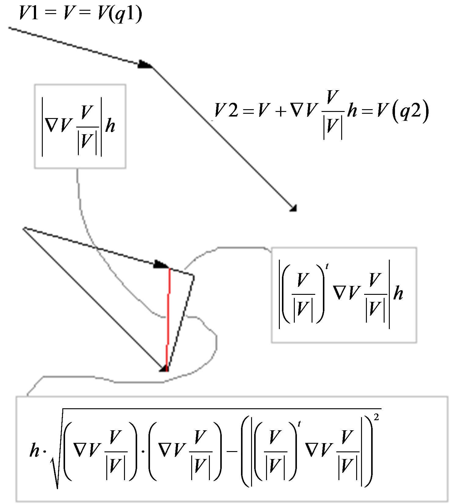
Figure 2. “Bending Energy” which is the Field Curvature multiplied by the squared norm of the gradient and its Euclidean geometric meaning—how much the field changes in direction perpendicular to itself.
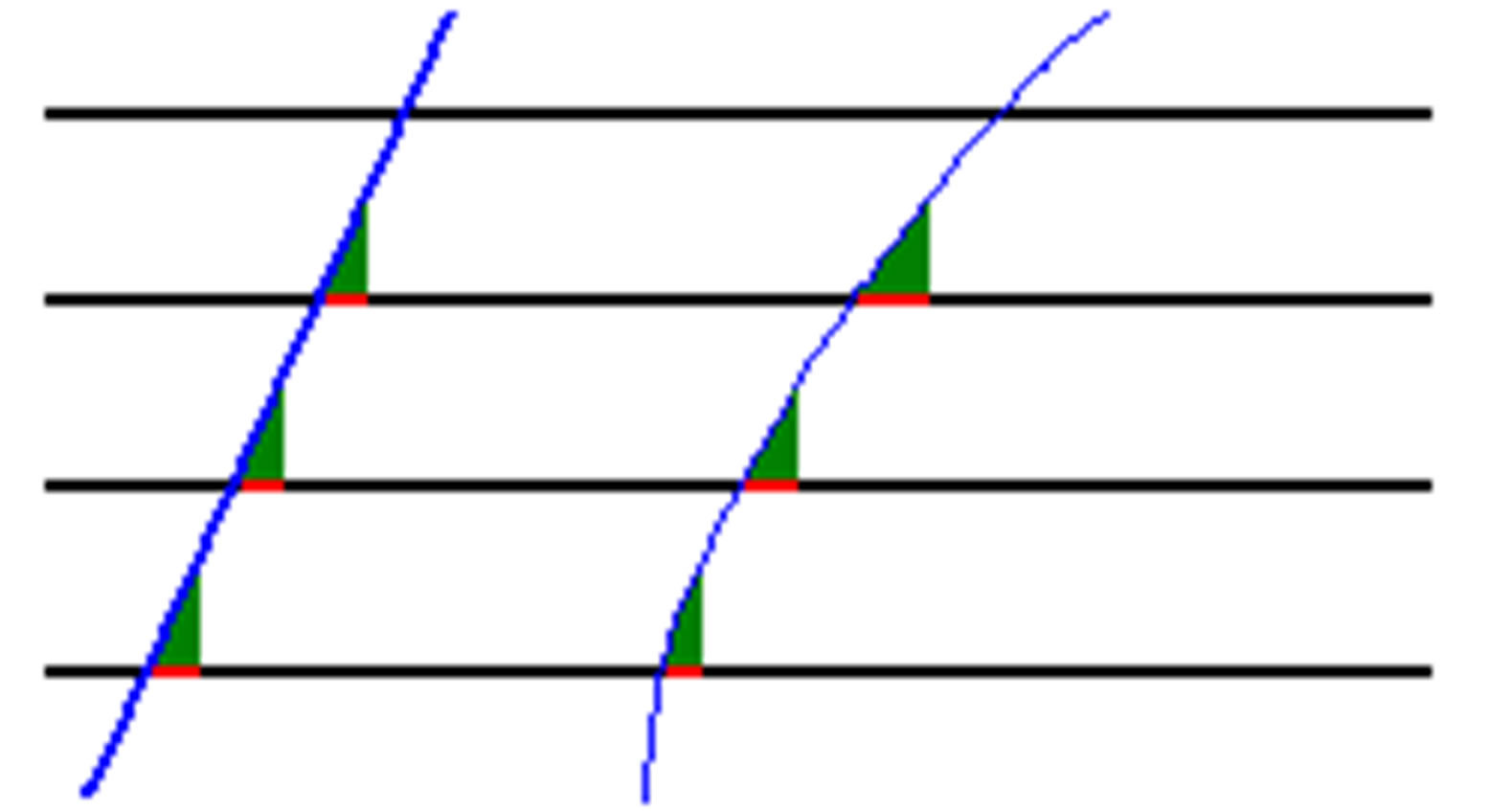
Figure 3. Parallel deviation on the right.
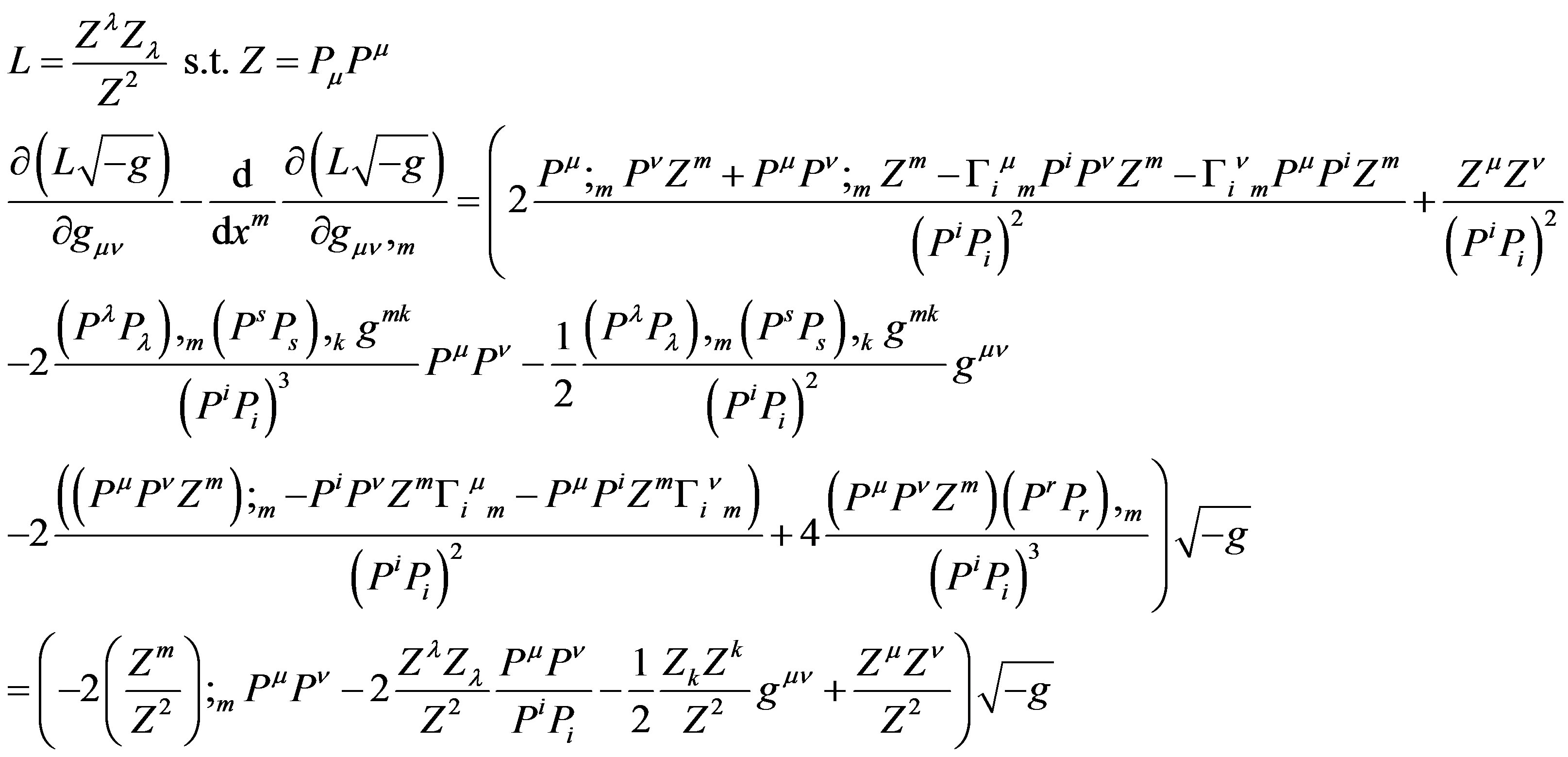
3. Tensor Formalism of the Square Curvature
As will be discussed, in tensor formalism, derivatives are replaced by covariant derivatives and are denoted by semi colon and derivatives by comma. Upper and lower indices represent the covariant and contra-variant properties and upper and lower indices sum according to Einstein convention so (2) can be written as a tensor density with local coordinates in . We will also divide (2) by
  in order to achieve a fully geometric action operator. Regarding the square root of the determinant of the metric tensor
 , following are tensor densities [6], that yield tensor equations [7],
 (3)
(3)
that can be written as 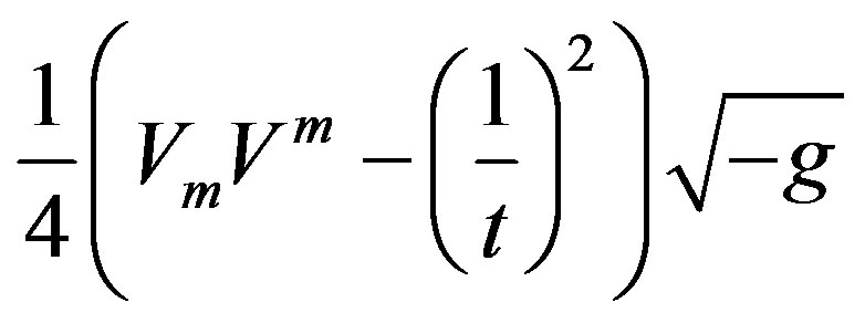 for
for
 and
and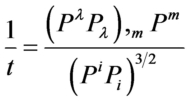 .
.
and  for coordinates
 . If P is the upper limit of measureable time from near big bang to any event then (3) is the second power of the curvature of the gradient
 .
.
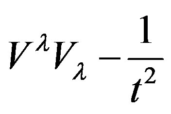
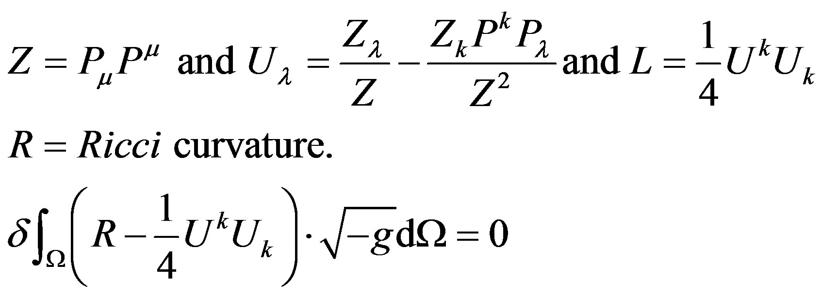
Don’t confuse the scalar function  with maximum proper time. We choose a simpler expression for our upper limit from near “big bang”, namely
 , and where there is no matter in space-time we expect one of the following to be true.
 (4)
(4)
 . (5)
. (5)
(4) is offered for a deterministic theory and (5) for quantum.
Please note that Square Curvature (P) = Square Curvature (kP) for constant .
.
Please note that in the model presented in (5), the time  is coupled with a wave function
  and there is only a need for
 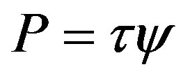 to have 3rd order derivatives but not for
  alone. The formalism of (5) possibly needs multiplication by
 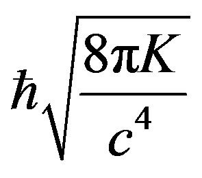 for each differentiation, such that K is the constant of gravity and
  is the Planck constant divided by
 .
.
Repeating our question: Can  be non-tangent to a geodesic curve:
1) If there is more than one geodesic curve that connects the “Big Bang” event to say event “e”, then obviously  need not be geodesic in a small neighborhood of “e”.
2) Intersection of different curves if coordinates are uncertain in quantum sense.
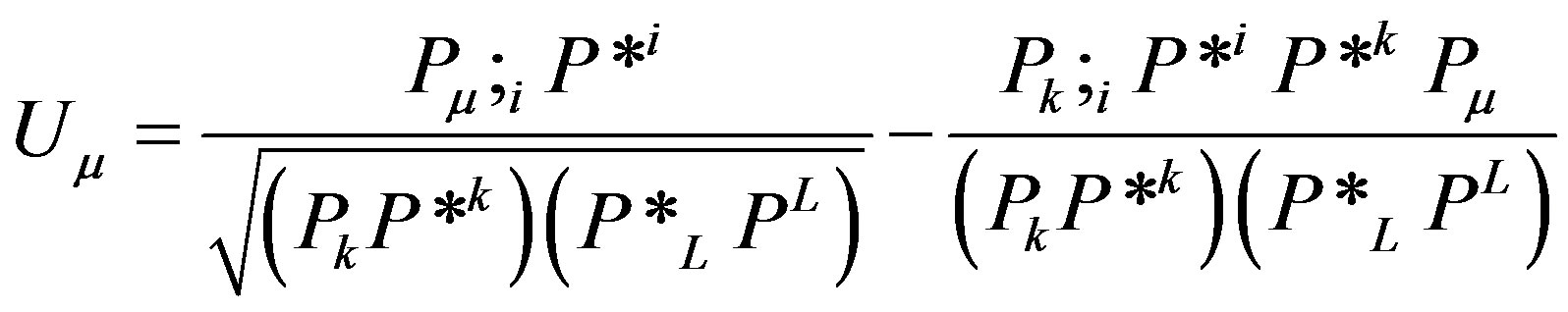
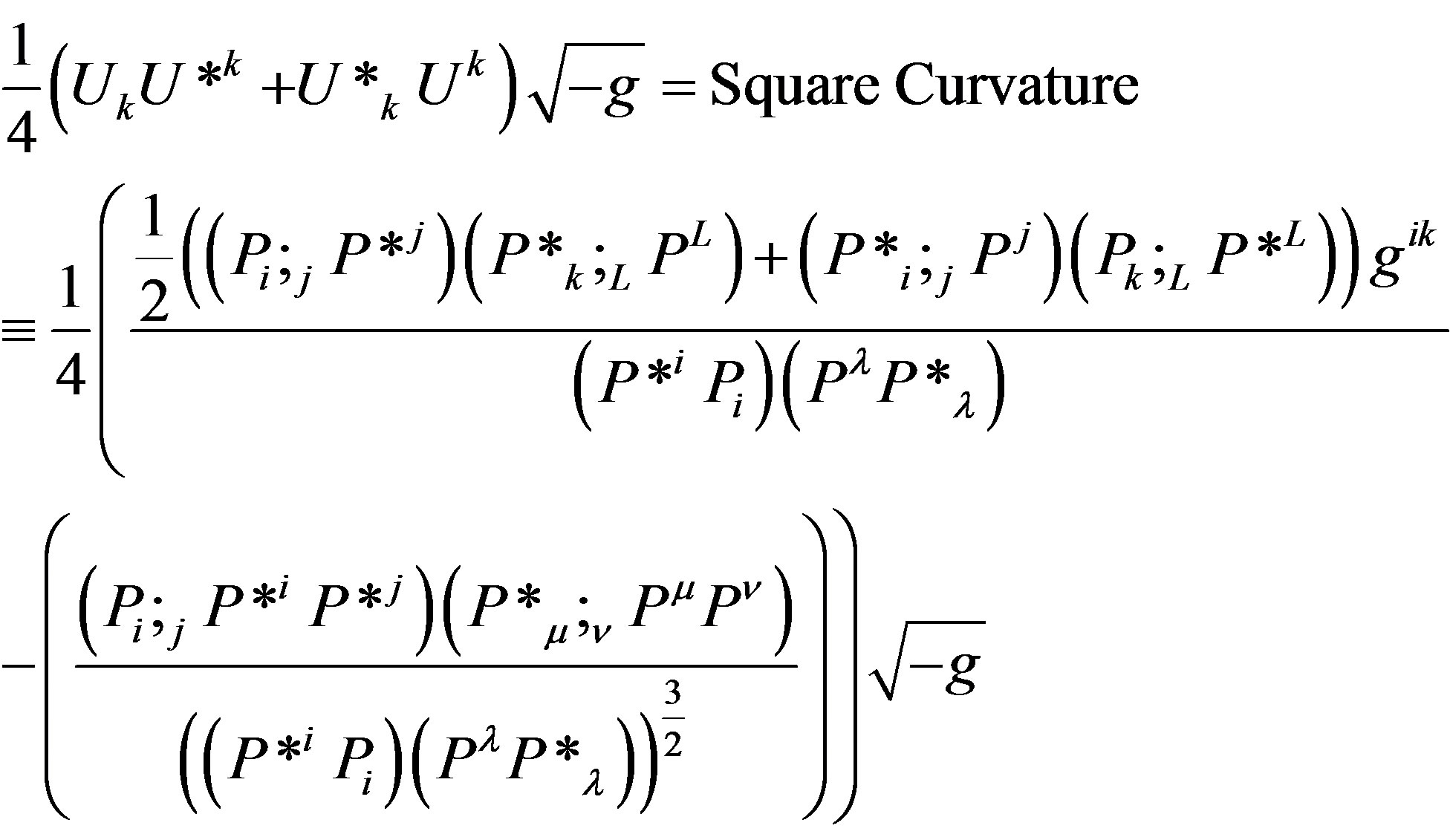
Development of (3) can be from the following:
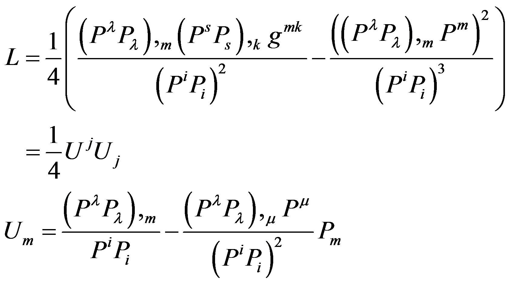 (6)
(6)
Obviously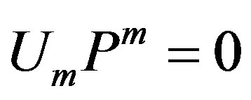 . The vector
  describes the direction and intensity of the curvature of the field
  which is a change perpendicular to
 .
.
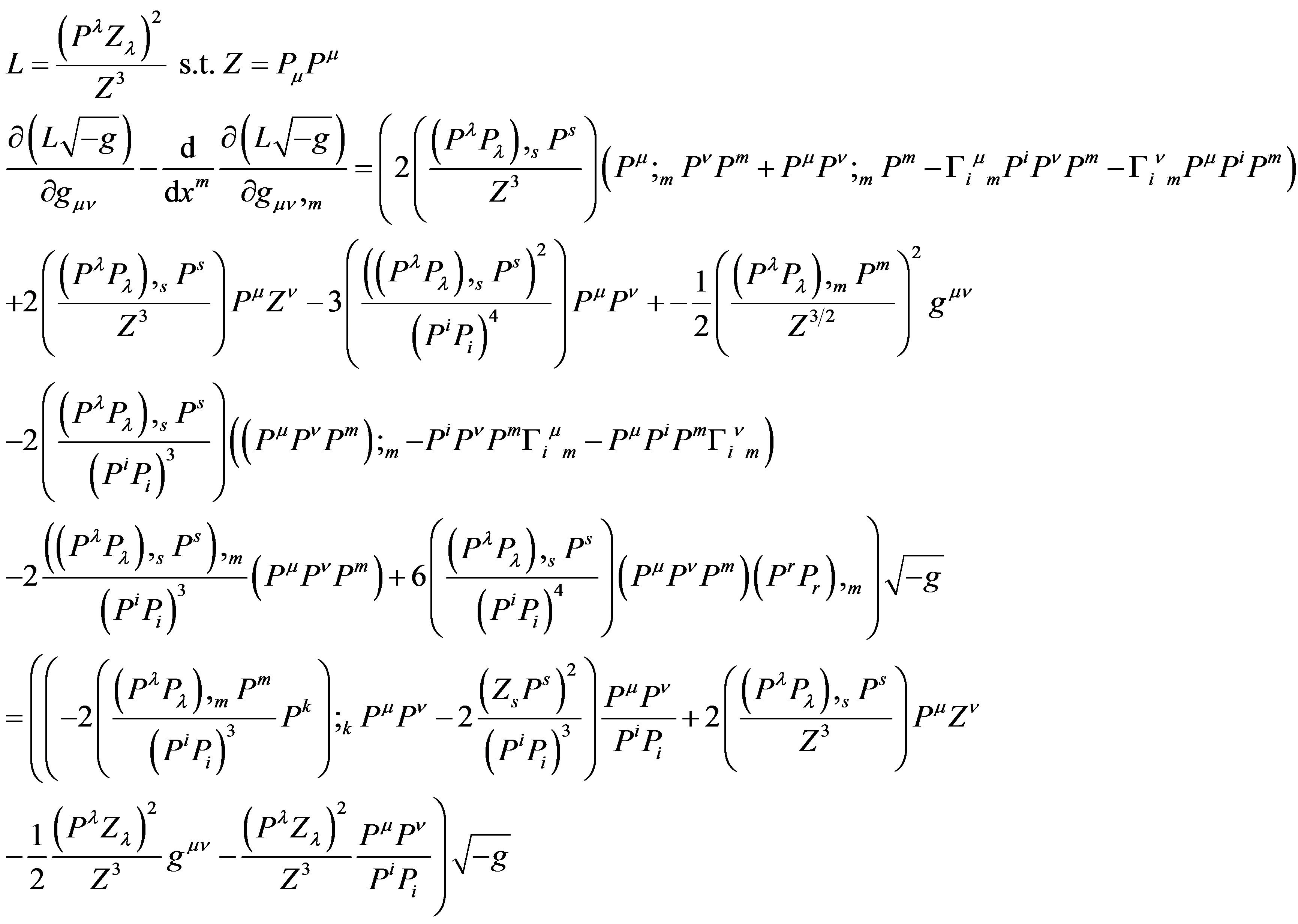
From minimum action of

See Appendix A,
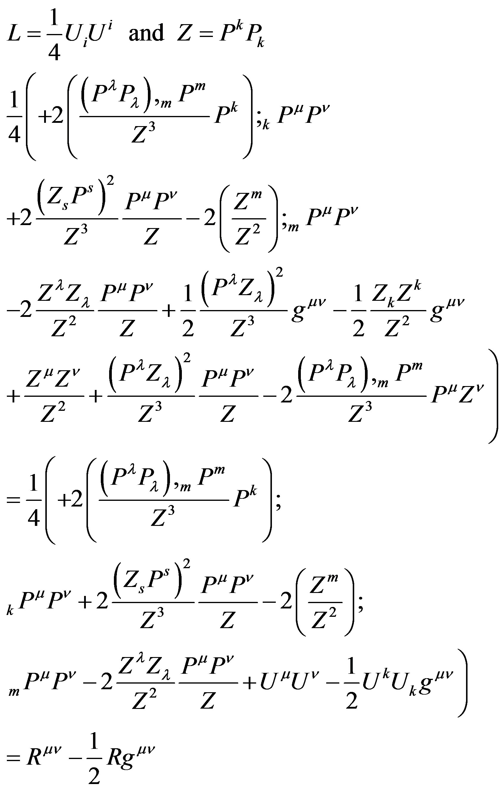 (7)
(7)
as we shall see later, a simple solution to the Euler Lagrange equations by  and it’s derivatives yields

and
 (8)
(8)
and therefore (7) becomes
 (9)
(9)
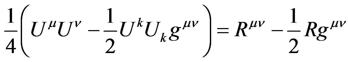
and we have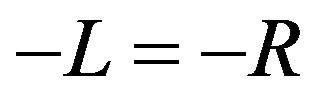 , such that
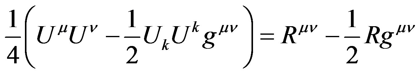
  is the Ricci curvature tensor [8,9]. If we ignore (6), and the coming (18)-(24) and (34)-(36), it is a bit disappointing that after all the efforts we simply get [8,9] which look like an ordinary General Relativity matter-geometry equation. There is always a way to solve the following equation
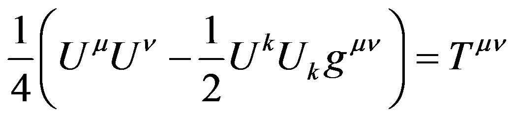 for an ordinary dust energy momentum tensor and therefore (9) is consistent with existing theories and is an important link to well established work on General Relativity.
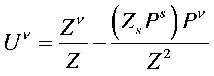
In other words, curvature of the gradient of the upper limit of measurable time from near “Big Bang” to an event is equivalent to Ricci curvature. If that is true then we can have an equation that is based solely on geometry. In any case we have a nice action (without spinors [10] and other advanced mathematical technology, though 4-force means rotation) of the form:
 such that
  is a vector field and
  is a scalar field. If the definition is in 3 dimensions, it hints at 4 dimensional Lorentzian metric geometry.
  is in units of
 . For the complex square (second power of) curvature operator we set the curvature vector
 .
.
Obviously . Bearing in mind that in our case
 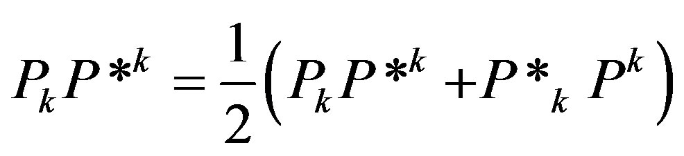 we calculate
 (10)
(10)
4. Quantum Gravity in a Nutshell
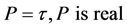
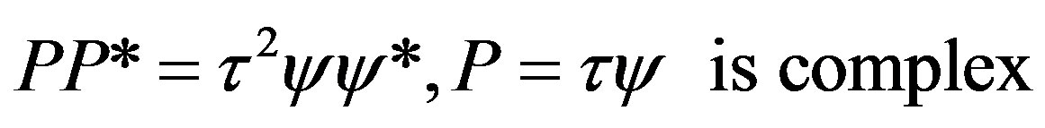
The observable in the offered theory is a scalar field of time. Time can be either , or
, or  where the theoretical formalism is the complex formalism (of Square Curvature) although (10) is incomplete without multiplication of each derivative by
 . The change in the direction of the gradient of the time field is due to the need to avoid discontinuity of gradient measurement by particle clocks in max proper time curve intersections. Discontinuity of the gradient is avoided by uncertainty of the intersection events/strings. Then
  could be the probability of the 4-location of such avoided geodesic conflict in the middle of a constellation of particles. The coupling of
  and
and  has one important meaning which is that quantum uncertainty resolves the discontinuities of the gradient of
  and prevents its measurement. In the classical model of gravity in this theory,
  is “smoothened out” by the Equation (7) or (9) which is an approximation or a limit of a Quantum effect. The classical model is sufficient for a giving a new description of matter, however,
  is required for resolving gradient singularities of
  that do not exist in the classical model.
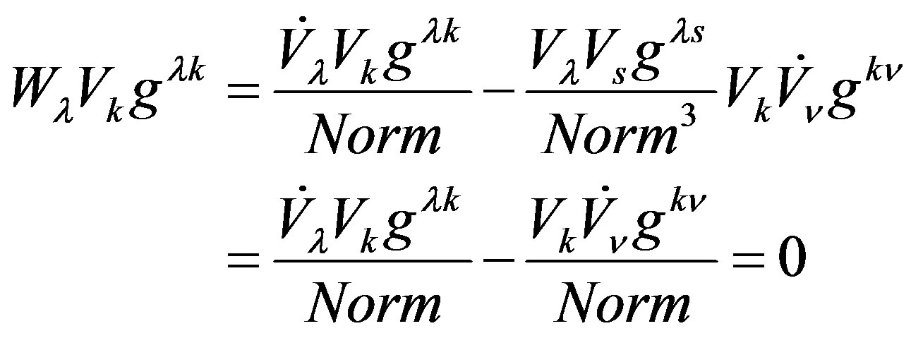
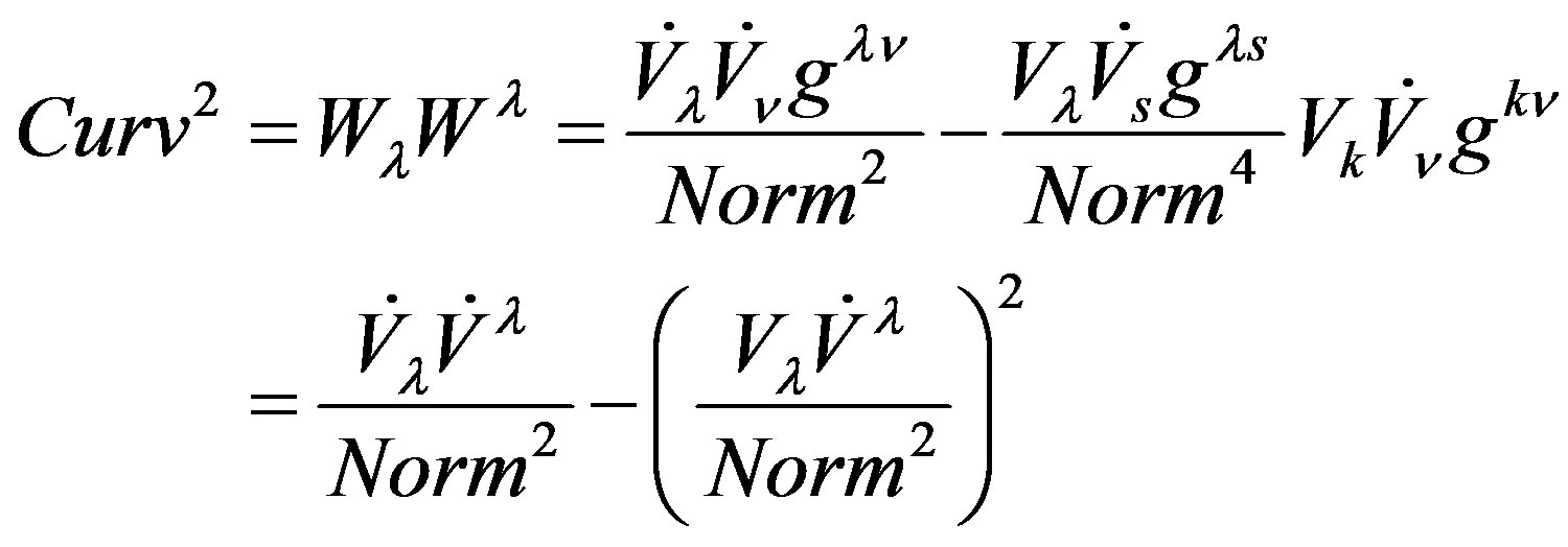
5. Proof That Square Curvature Is the Square (to the Second Power of) Field Curvature
We restrict the proof to the Euclidean case. The square curvature is defined as
 (11)
(11)
such that  is a diagonal unit matrix. For convenience we will write
  and
and . For some parameter
 . Let
. Let  denote:
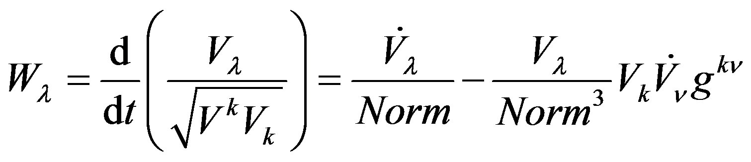 (12)
(12)
Obviously
 (13)
(13)
Thus
 (14)
(14)
Since  is the derivative of the normalized curve or normalized “speed”,
such that  denotes the local coordinates.
If  is a conserving field then
  and thus
 (15)
(15)
Writing the last term in Riemannian geometry is the same field curvature operator that we chose.
6. Byproduct—Separable Coordinates Where the Time Coordinate Is Parallel to at Least One of the Global/Absolute Maximum Proper Time Curves
The following is a bit speculative but may be important. We see that 3 dimensions hint at 4 dimensional action. This is done by looking at the action (3) in three dimensions and observing the following way to write it,
 (16)
(16)
where  is the metric tensor in 4 dimensions and
  is in 3 dimensions.
  implicitly refers to a local submersion [11] where time is locally held constant.
Can we do the opposite, look at 4 dimensions and reduce the problem to 3 without violating the principle of covariance?
First, our upper limit proper time curves are intrinsic and do not depend on the coordinates unless more than one curve intersect with the same event.
We can therefore agree that the absolute maximum proper time curves are different than ordinary geodesic curves on which only local maxima of proper time can be measured.
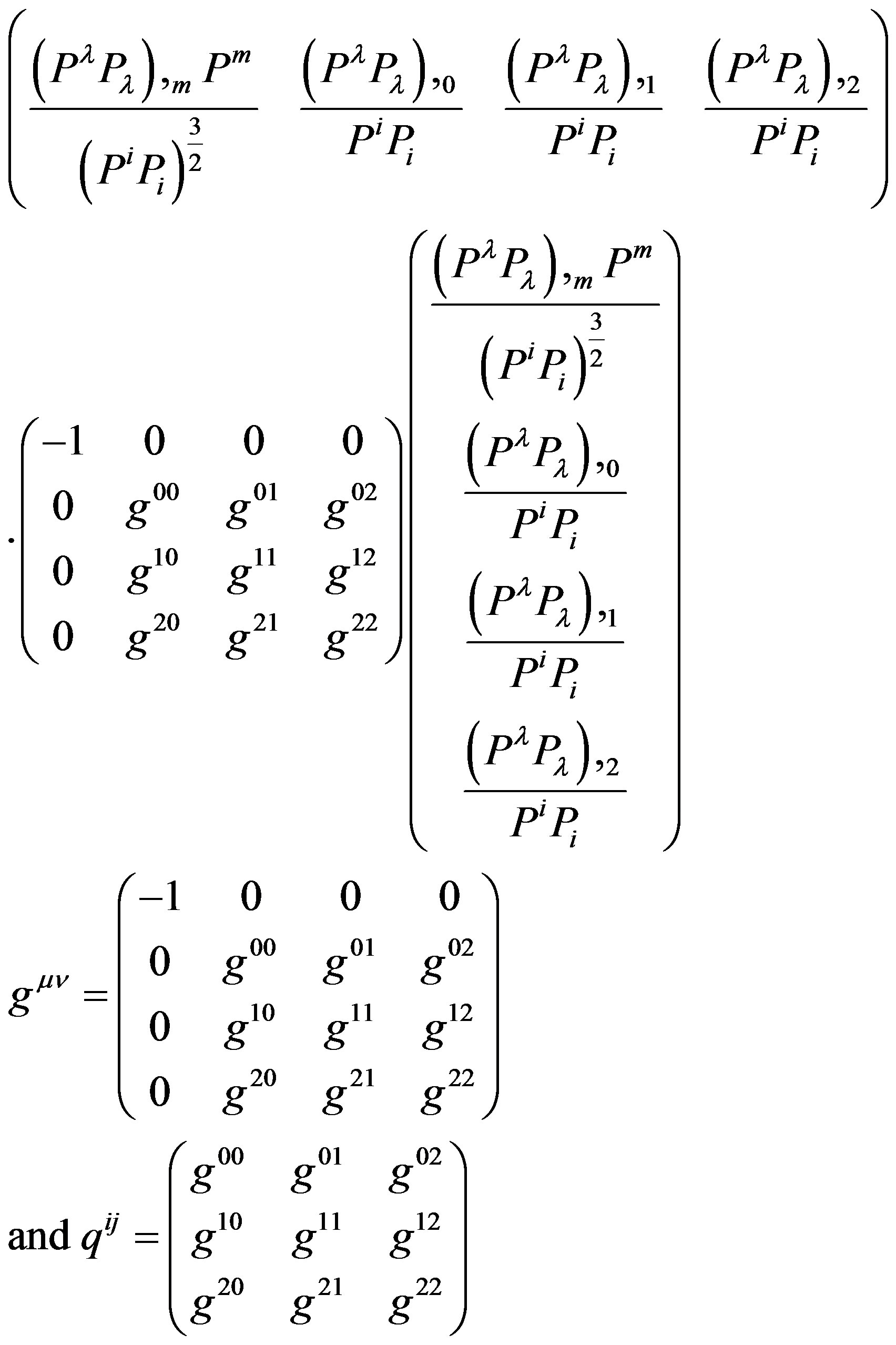
We choose to describe (3) on our space-time in our special coordinates. Under correct local choice of coordinates, the direction in space time of the maximum proper time is an eigenvector of the metric tensor with the biggest eigenvalue, our metric tensor is of the form presented in (16) for which the mixed space time terms are zero. Also,

and

Please note: We can assume as possible
 especially if multiple maximum proper time curves to the same event “e” exist. Instead of (3) we reduce the action to become three dimensional,
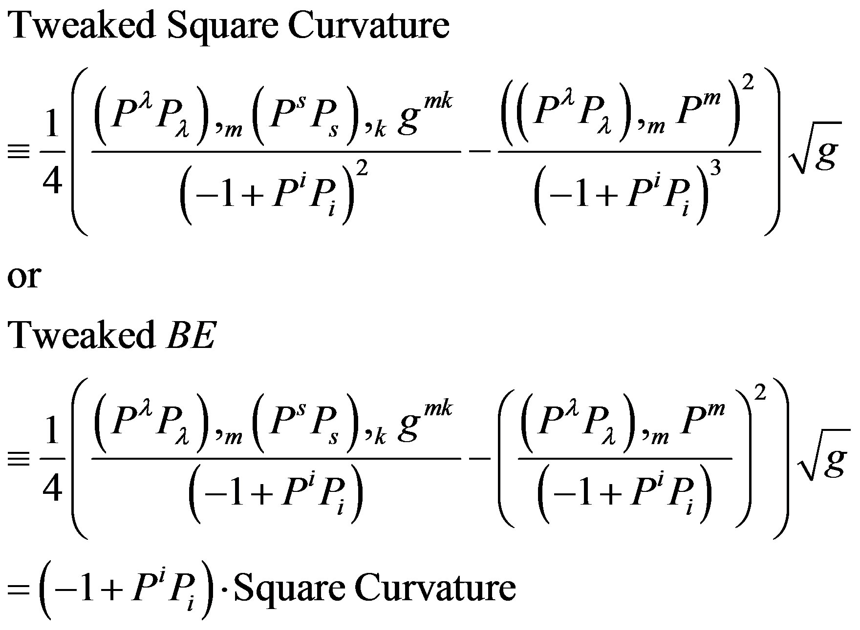 (17)
(17)
This means that on our three dimensional sub-manifolds (“Leaves of a foliation”), there is a corresponding action operator that is free of derivative dependence on time.
Solving the Euler Lagrange equations for the Tweaked Square Curvature and receiving a plurality of solutions is indeed a promising direction of research!
7. Unsynchronizability
Since  is not constant on the 3 dimensional submanifolds perpendicular to the global/absolute maximal proper time curves, these manifolds are not synchronizable and are therefore not the ideal inflating S(3) i.e. Friedmann-Robertson-Walker.
8. History of the Paper’S Concept of Time
The idea of an absolute time, such as maximum proper time from a common event, i.e. “big bang” is not new [12,13] and it appears in Hebrew writing such as the Book of Principles by Rabbi Josef Albo 1380-1444. Rabbi Josef Albo wrote about time that can be measured by devices and another aspect of time which he termed immeasurable. The maximum proper time can’t be measured by devices on Earth because due to General Relativity, clock ticks are slowed down by the gravitational field. It is an upper limit.
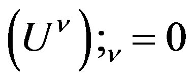
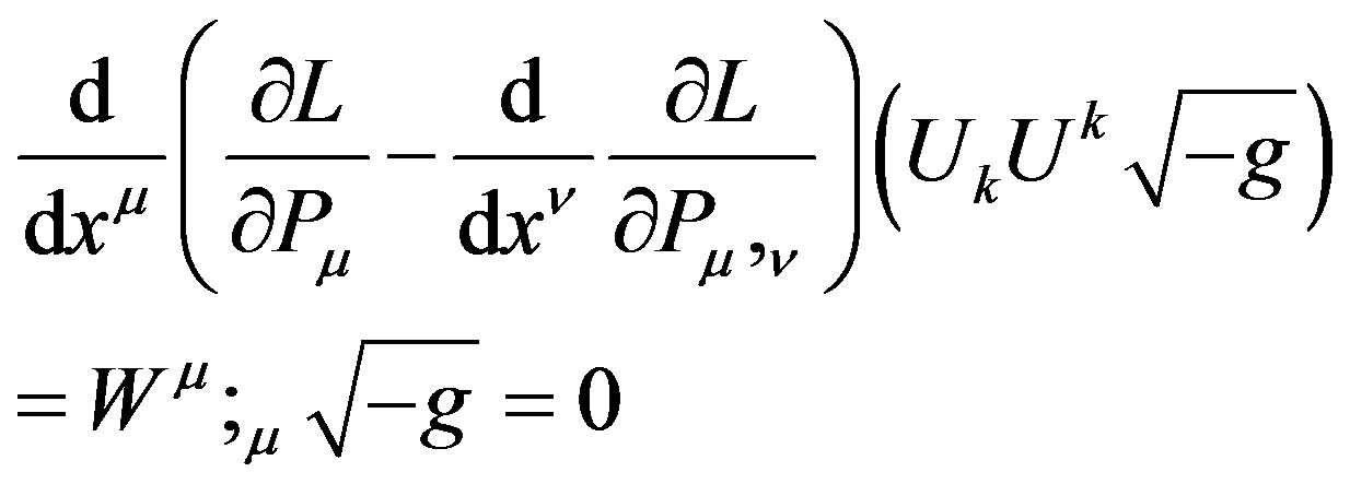
9. Conservation of Known Matter from the Euler Lagrange Equations
Finally we get the following zero divergence:
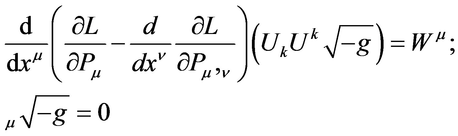
where
 is obtained from the subtraction of (35) from (36), see Appendix A.
Variation by  and its derivatives is a special case
 .
.
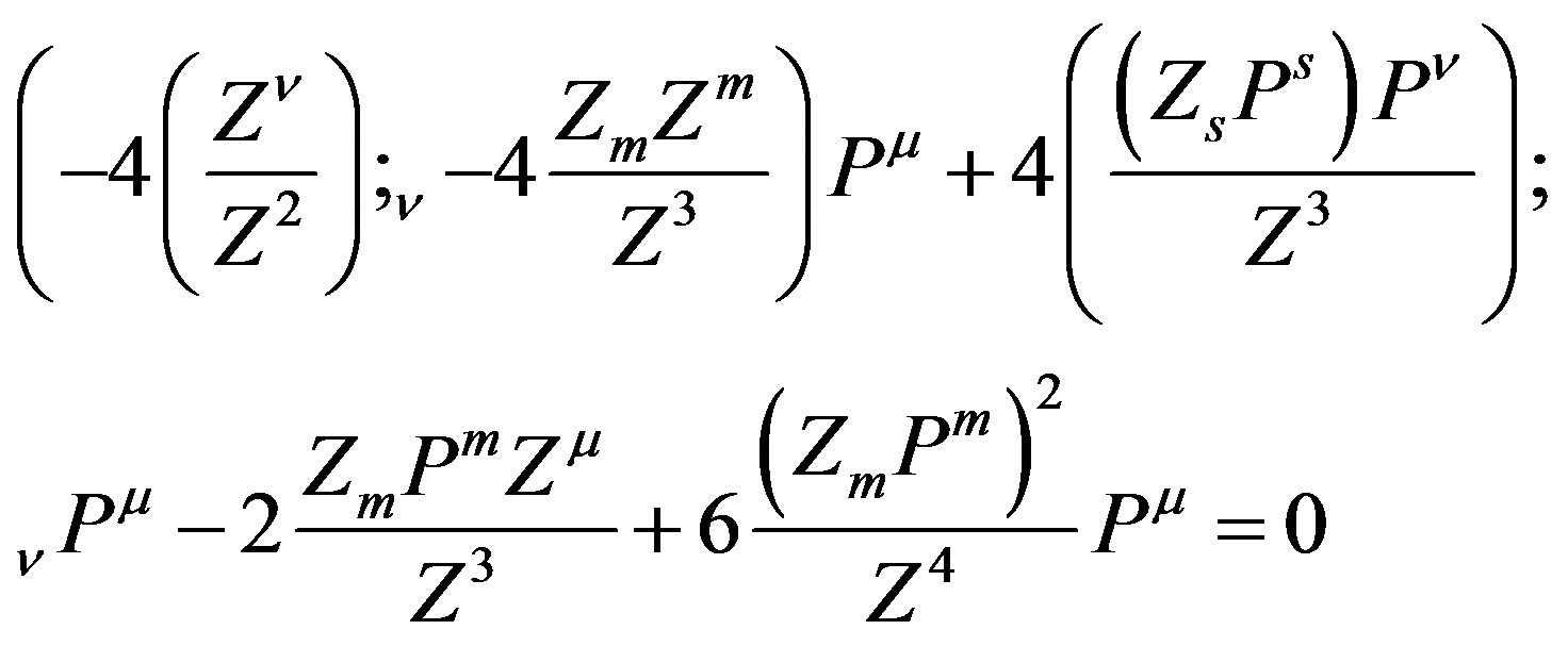 (18)
(18)
Multiplication by  and contraction yields,
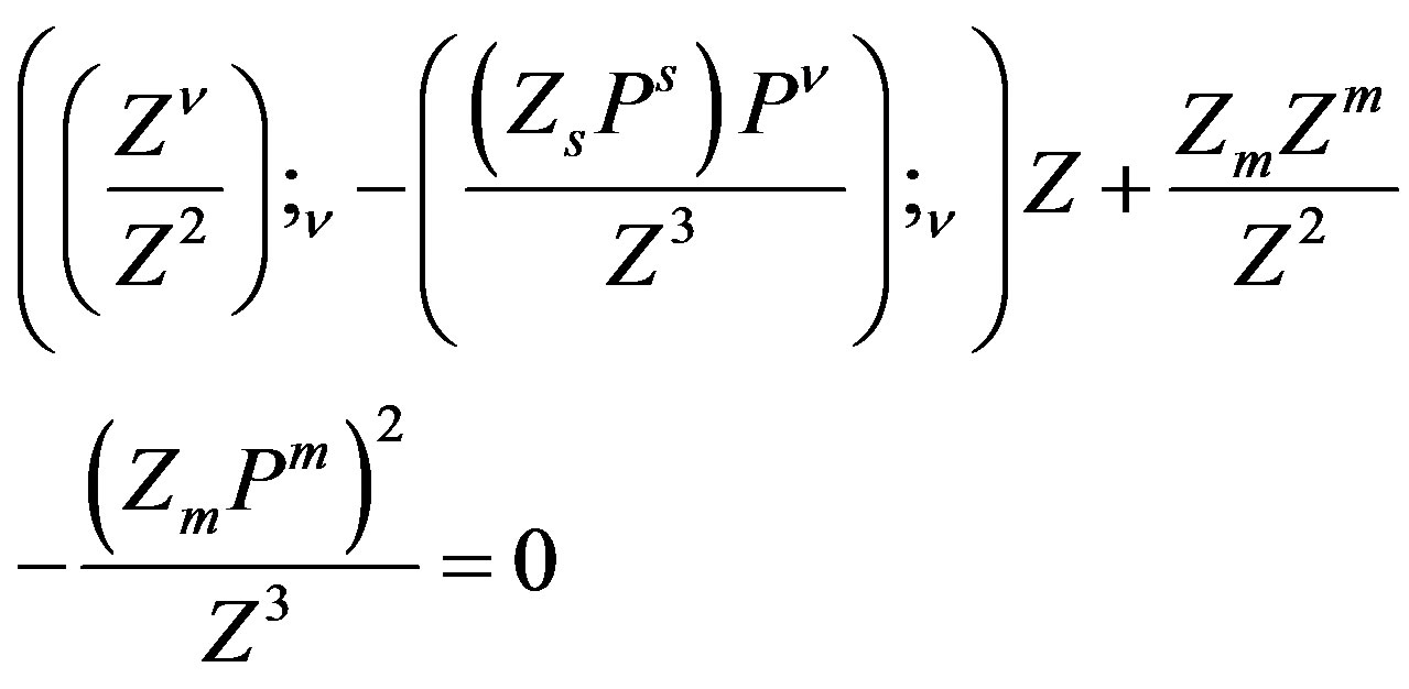 (19)
(19)
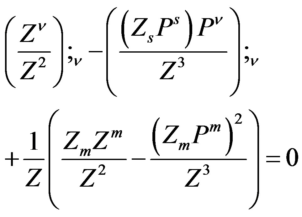 (20)
(20)
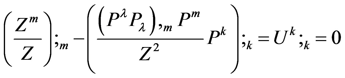
and as a result of (20) the following terms from (7) vanish,
 (21)
(21)
Which yields a simpler Equation (9). Recall that
 And that
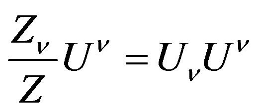
 (22)
(22)
Which proves (8)
 (23, see 8)
And proves the simple representation of the field equations That we saw in (7)
 (24, see 9)
10. Chameleon Fields or Pressure?
As we can see, the more general case is,
 (25)
(25)
 (26)
(26)
instead of
 (27)
(27)
An effect which is contrary to gravity will add a positive delta to the Ricci curvature and therefore from (7), multiplication by the metric tensor  and contraction yields,
 (28)
(28)
An effect which adds gravity, will add negative delta to Ricci curvature and therefore,
 (29)
(29)
Known matter will be simpler
 (30)
(30)
It is possible that either (28) or (29) is mathematically not valid. Additional terms can’t violate the vanishing of the divergence of Einstein tensor.
If one of them is correct then there is a particle which its force fields decay very fast with distance, in other words, discovery of weakly interacting particles may imply either (28) or (29).
High order derivatives of the metric tensor and pressure were studied by Deser and Tekin [14]. For application of (28) and/or (29) to space-time warp drive please refer to [15].
11. Acknowledgements
I would like to thank my boss, Mr. Yossi Avni for approving my idea of using Riemannian geometry and a curvature operator in minimum cost functions in the company’s research of hand signature recognition. His approval lead not only to new technology but also to this paper. I also would like to thank him for helping me to prepare a poster for an Israeli physics conference IPS 9, December, 2012.
Thanks also to supporters of this theory, Dr. Sam Vaknin who presented to me the idea of Chronons as clock particles and to Professor Larry (Laurence) Horwitz whose advices were very useful. My special thanks to emeritus professor David Lovelock for his help in corrections of the Euler Lagrange equations several years ago.
12. Conclusions—Test to the Theory
12.1. General
Maximal time is measured by particles. This time sets an upper limit on measurable time quite similar to the way the speed of light sets an upper limit on speed. Since time is measured by material clocks, these material clocks are influenced by forces. The particle that can measure the maximal possible time from the “big bang” to an event within matter will therefore be influenced by such forces. For the trajectory to be meaningful, either there exists a force which can’t be gravity since gravity is not a force, such that the force will depend on mass or that only a unique particle can enter the force field. Evidence of mass dependent force will be shortly discussed. Such an effect can also attest to gravity and it is therefore difficult to distinguish between the two.
Although the upper limit of measurable time is measured along curves, the gradient of that time is local, which makes the use of such scalar field feasible to theoretical physics.
Non geodesic motion as uniform acceleration is well defined by Friedman-Scarr representation and has a linear interpretation by an anti-symmetric tensor [16] which also indirectly describes a more intuitive alternative to spinors (well at least if we can blissfully afford to ignore wave functions, and group representation), however, the most interesting effects that this theory offers, are beyond the scope of Friedman-Scarr representation of acceleration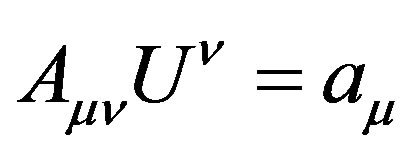 , speed
  and acceleration matrix
 .
.
12.2. Unconventional Conclusions
There is experimental evidence regarding high gradient of an electric field in which force that acts on metal balls is represented as the ordinary force on the induced dipole as in ordinary dielectrophoresis plus an unexpected “force” that depends on mass [17]. [17] can attest to the existence of true force field, which is not gravity, that depends on mass, as also seems to be an outcome of this theory. This is one way to achieve a unique trajectory of the maximally measured proper time by any massive test particle including zero mass Chronons [1]. In this case, [17] can be a residual force of the original force field.
Another effect is that (28) and (29) allow gravity to be generated from non linear force fields. If the 4-force is not linear then (28) or (29) are possible which allow warps or gravitational dipoles [15]. In order for such an effect to be consistent with the vanishing divergence of Einstein tensor and with conservation laws, (28) and (29) mean the creation of gravitational dipoles. The overall momentum—energy must be preserved.
In this case, the simple Equation (7) can’t be reduced to (9).
REFERENCES
- S. Vaknin, “Time Asymmetry Revisited [microform],” Ph.D. Dissertation, Library of Congress, Microfilm, 1982.
- J. W. Milnor, “Topology from the Differentiable Viewpoint,” Princeton Landmarks in Mathematics, Princeton University Press, Princeton, pp. 32-41.
- J. N. Munday, F. Capasso and V. A. Parsegian, Nature, Vol. 457, 2009, pp. 170-173. doi:10.1038/nature07610
- V. Guillemin and A. Pollack, “Homotopy and Stability,” Differential Topology, Princeton Landmarks in Mathematics, Princeton University Press, Princeton, pp. 33-35.
- Y. Avni and E. Suchard, “Apparatus for and Method of Pattern Recognition and Image Analysis,” US Patent No: 7424462.
- D. Lovelock and H. Rund, “The Numerical Relative Tensors,” Tensors, Differential Forms and Variational Principles, Dover Publications Inc., Mineola, pp. 113- 114.
- D. Lovelock and H. Rund, “Tensors, Differential Forms and Variational Principles,” Dover Publications Inc., Mineola, pp. 323-325.
- D. Lovelock and H. Rund, “Tensors, Differential Forms and Variational Principles,” Dover Publications Inc., Mineola, p. 262.
- D. Lovelock and H. Rund, “Tensors, Differential Forms and Variational Principles,” Dover Publications Inc., Mineola, p. 261.
- E. Cartan, “The Theory of Spinors,” Dover Publications Inc. Mineola, p. 149.
- V. Guillemin, “Submersions, Local Submersion Theorem,” Differential Topology, Princeton Landmarks in Mathematics, Princeton University Press, Princeton, p. 20.
- Rambam, “The Guide For The Perplexed By Moses Maimonides (Moreh Nevuchim), Part. II, Chapter 13,” Routledge and Kegan Paul Ltd., London, 1904.
- J. Albo, “Immeasurable Time-Maamar 18, measurable, Time by Movement,” Book of Principles (Sefer Haikarim), Chapter 2, Chapter 13, (Circa 1380-1444, unknown), The Jewish Publication Society of America 1946.
- S. Deser and B. Tekin, Physical Review Letters D, Vol. 67, 2003, Article ID: 084009. doi:10.1103/PhysRevD.67.084009
- M. Alcubierre, Classical and Quantum Gravity, Vol. 11, 1994, pp. L73-L77.
- Y. Friedman and T. Scarr, Physica Scripta, Vol. 86, 2012, Article ID: 065008. doi:10.1088/0031-8949/86/06/065008
- T. Datta, M. Yin, A. Dimofte, M. C. Bleiweiss and Z. Cai, “Experimental Indications of Electro-Gravity,” 2005. arXiv:physics/0509068 [physics.gen-ph]
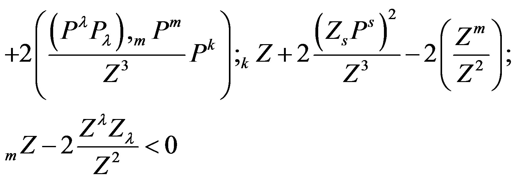
Appendix A: The Euler Lagrange Equations of the Square Curvature Action
We will not solve the entire system
 (31)
(31)
But rather focus on 
 (32)
(32)
 (33)
(33)
 (34)
(34)
 (35)
(35)
 (36)
(36)
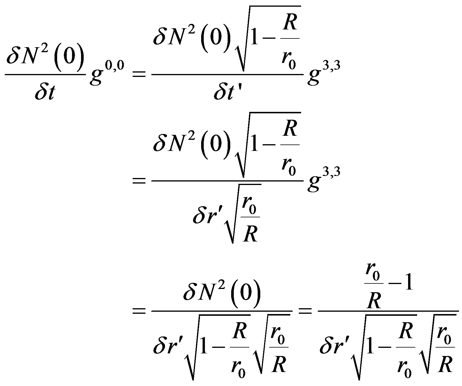
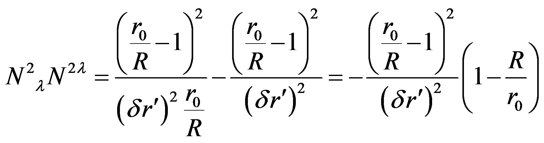
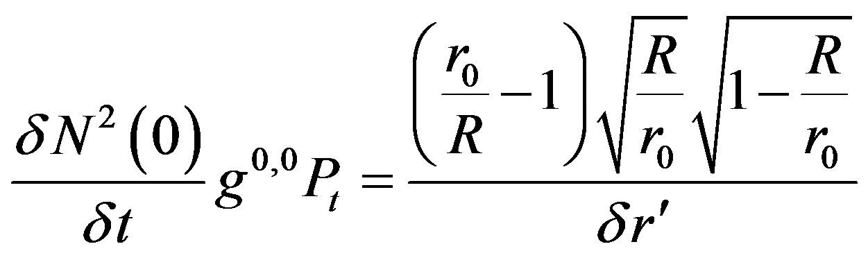
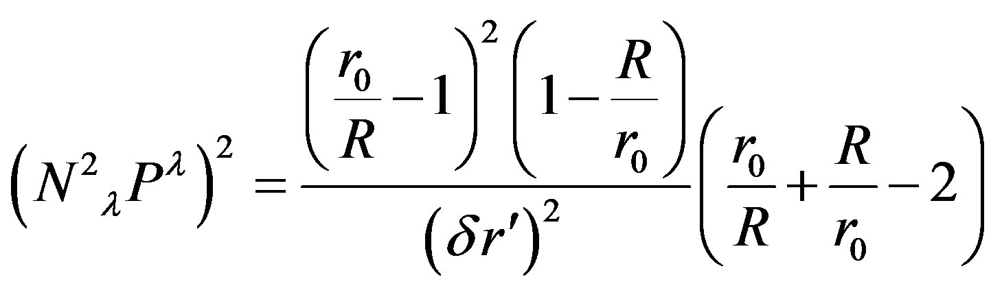
Appendix B: The Scalar Time Field of the Schwarzschild Solution
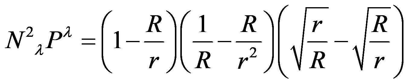
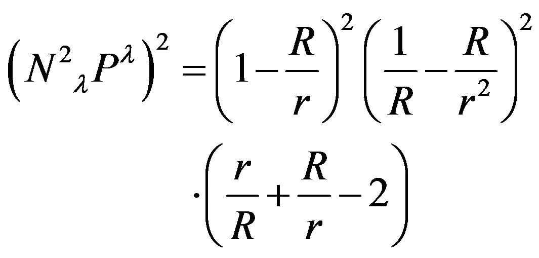
We would like to calculate

in Schwarzschild coordinates. This theory predicts that where there is no matter, the result must be zero.
The result also must be zero along any geodesic curve but in the middle of a hollowed ball of mass the gradient of the absolute maximum proper time from “Big Bang” derivatives by space must be zero due to symmetry which means the curves come from different directions to the same event at the center. Close to the edges, gravitational lenses due to granularity of matter become crucial.
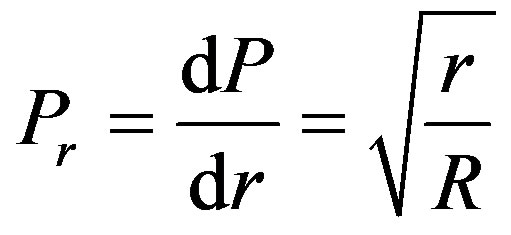
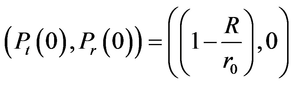
The speed  of a falling particle as measured by an observer in the gravitational field is
 (37)
(37)
where  is the Schwarzschild radius. If speed
  is normalized in relation to the speed of light then
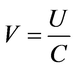 .
.
For a far observer, the deltas are denoted by  and,
and,
 (38)
(38)
because  and
and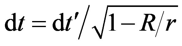 .
.

Which results in,
 (39)
(39)
Please note, here  is not a tensor index and it denotes derivative by
On the other hand

Which results in
 (40)
(40)
Please note, here  is not a tensor index and it denotes derivative by
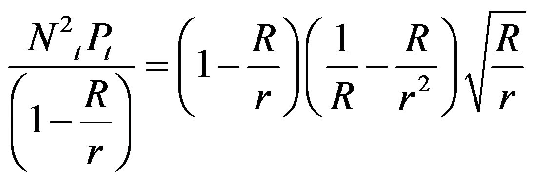
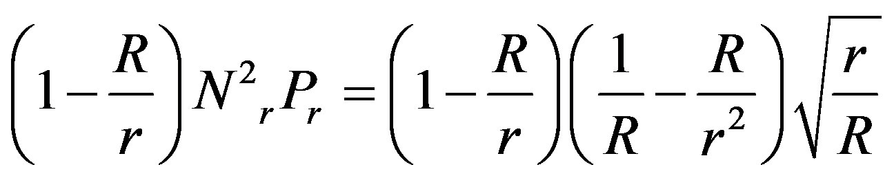
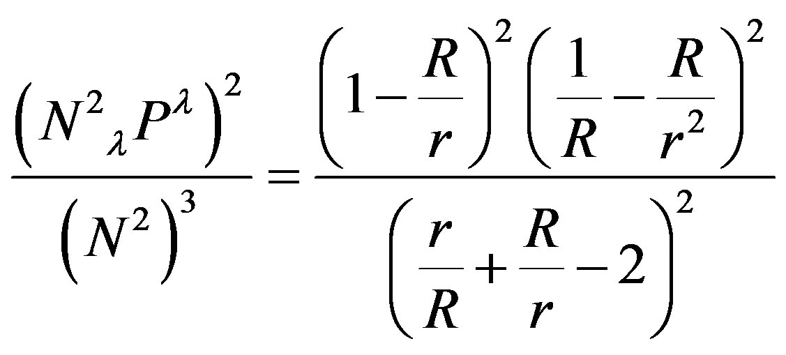
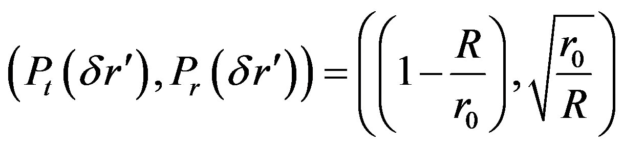
For the square norms of derivatives we use the inverse of the metric tensor, So we have
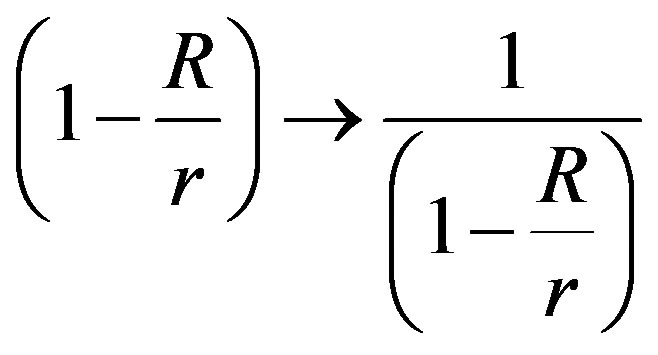 and
and 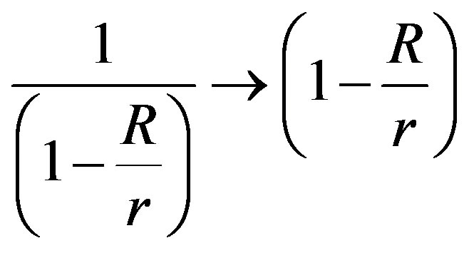
So we can write
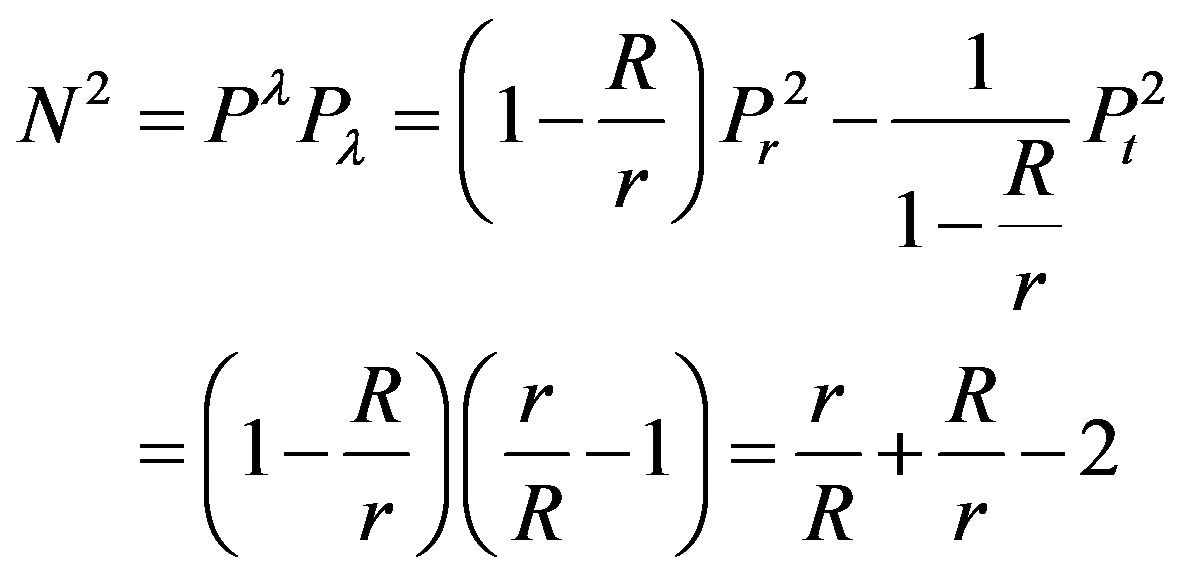
 (41)
(41)
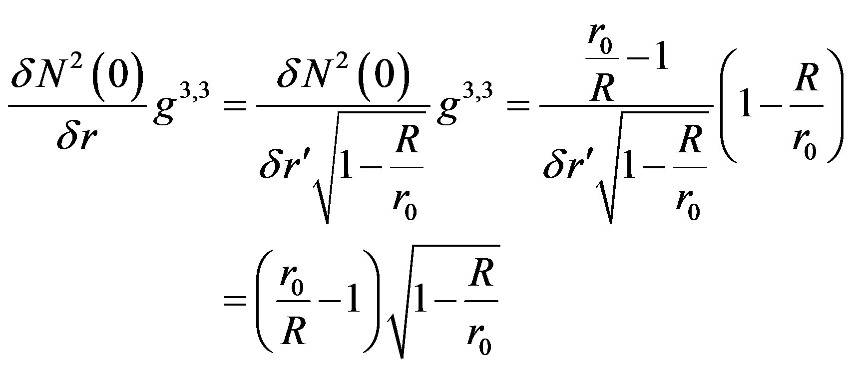
 And we can calculate
 (42)
(42)
We continue to calculate

and
 (43)
(43)
Please note, here  is not a tensor index and it denotes derivative by
 (44)
(44)
Please note, here  is not a tensor index and it denotes derivative by
and
 (45)
(45)
So
 (46)
(46)
And finally, from (42) and (46) we have,
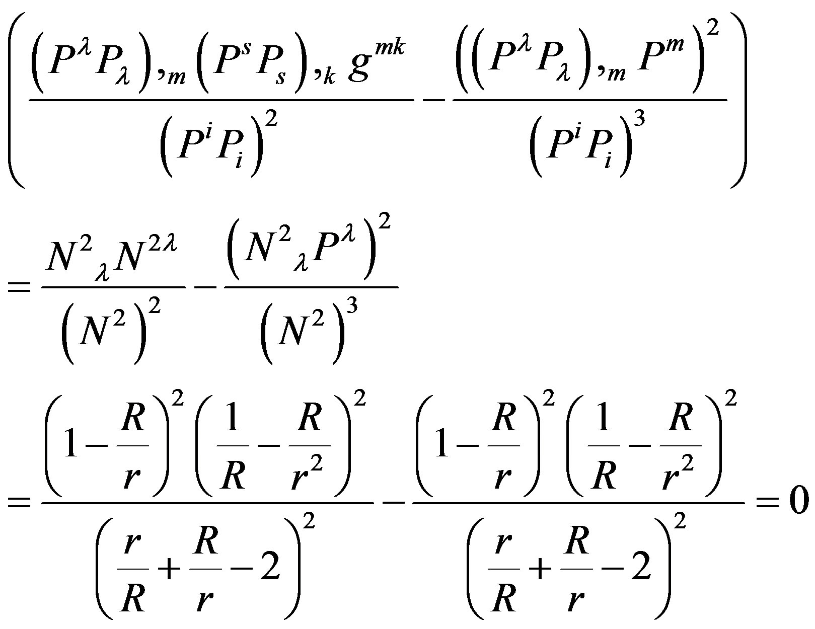 (47)
(47)
Which shows that indeed the gradient of time measured, by a falling particle until it hits an event in the gravitational field, has zero curvature as expected.
The term 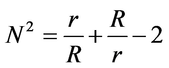 is slightly disturbing because at very far distances,
  becomes significant.
Moreover, if  has a lower atomic limit, then for such
 the term
 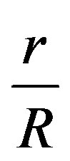 is a whole number We now return to the discussion about a hollowed ball of mass.
It is clear that the maximum proper time from “Big Bang” curves entering the ball are symmetrical in relation to the center and therefore

where  is the radius in the far coordinate system of the hollowed ball of mass. However,
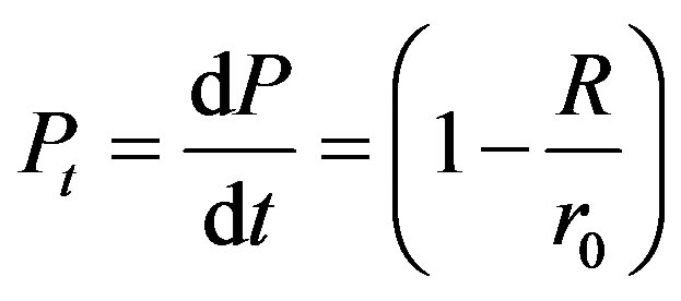 .
.
Writing the gradient in two dimensions in t, r, ignoring the gravitational lenses due to mass granularity, and ignoring quantum uncertainties of coordinates and of energy momentum, we have
 (48)
(48)
The last result  is an inevitable outcome of the symmetry in the center of the ball. The gradient by the space coordinates must be zero and the change of direction in the gradient means that curvature is inevitable.
Center analysis if there is an atom of movement length Without even negligible forces acting on a test particle and without quantum center location uncertainty, in the middle of a hollowed ball of mass the gradient of absolute maximal proper time is discontinuous due to symmetry. Suppose that the difference between the gradient at the center where  and where,
  , such that
  is small, results in
 . We want to measure the second power of the curvature of the gradient of absolute maximum proper time due to that difference. Suppose that the change happens smoothly within a small radius from the center, measured around
 .
.
We assume that such curvature measures how much the gradient is not geodesic due to curve intersections.
Consider  and
and 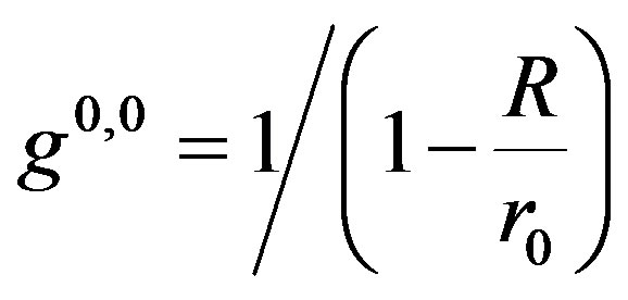
 (49)
(49)
 (50)
(50)
 (51)
(51)
 (52)
(52)
 (53)
(53)
 (54)
(54)
 (55)
(55)
 (56)
(56)
 (57)
(57)
 (58)
(58)
 (59)
(59)
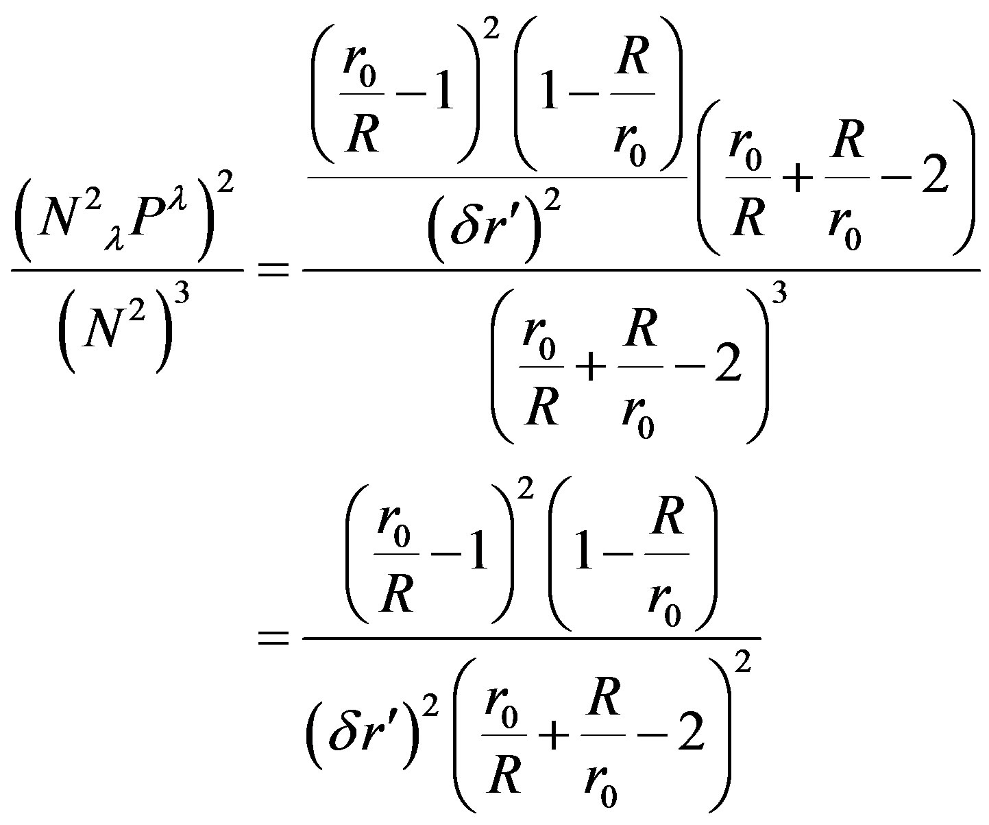 (60)
(60)
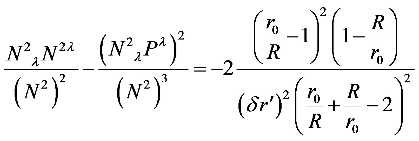 (61)
(61)
 (62)
(62)
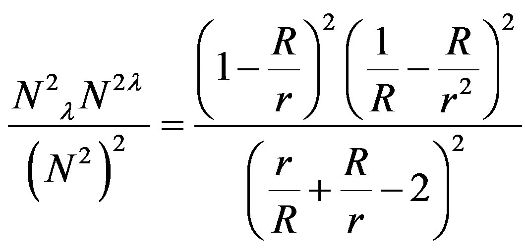
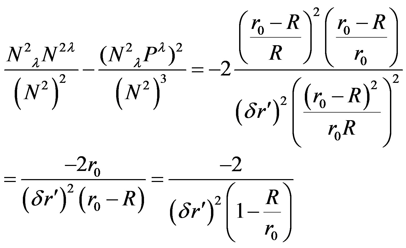
Given the radius  that is seen within the gravitational field, the surface of a small ball around the center is smaller than expected in flat space-time,
 (63)
(63)
We now calculate the curvature and then multiply it by the volume of the ball in which the direction of the gradient changes towards the center as seen in (49),(50),

 (64)
(64)
(64) is very interesting because it depends only on  and not on the mass of the gravitational source.
Appendix B2: Approximated Validity Test at the Planck Scale
(64) imposes some strict limits on the offered theory. For the following we assume that 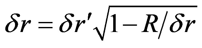 is big enough in comparison to the Schwarzschild radius R otherwise none of the following calculation will be validSuppose that all the matter we have is due to force field acting along the distance
 . Then by (9) and the following conclusion that
  and by Einstein equation of Gravity
 , and from (64) we have the following,
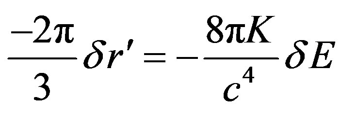 (65)
(65)
where 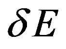 is achieved via integration of energy on space. K is the known Gravity constant
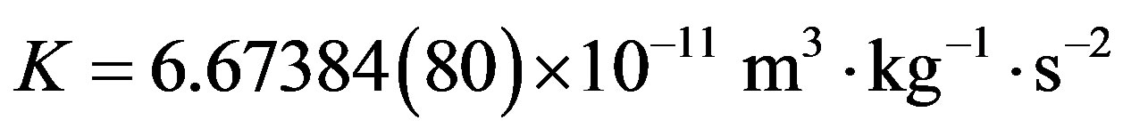
and
 .
.
So we can divide the equation by 
So we have
 (66)
(66)
That is quite a strong force, about
 Newtons.
On the other hand if our energy is within a ball of radius  and
and  is also the uncertainty of the space coordinate of the center then we have by the law of uncertainty of Quantum Mechanics
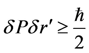 (67)
(67)
 and in the inequality extremity of equality,
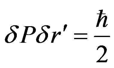 (68)
(68)
Now consider (66) which is a very strong force, acting on a small enough particle so virtually we can say that the speed of the particle is approximated by an average speed which the speed of light. So
 (69)
(69)
Recall the definition of work as Force multiplied by length on which the force acted, we have from (69) and from (66)
 (70)
(70)
This value is quite close to the Reduced Planck Energy which is defined as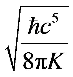 . and since it is smaller than Planck Energy
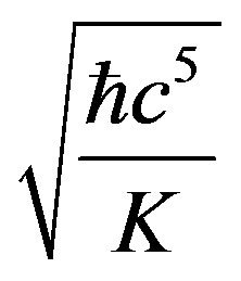 , our calculations imply that a single-photon black hole is highly unlikely to exist if there is a Planck length limit. Also pairs of photons will probably not create a microscopic black hole.