Applied Mathematics
Vol.07 No.17(2016), Article ID:72197,28 pages
10.4236/am.2016.717178
An Effective Numerical Calculation Method for Multi-Time-Scale Mathematical Models in Systems Biology
Yohei Motomura1, Hiroyuki Hamada1,2, Masahiro Okamoto1,2
1Graduate School of Systems Life Sciences, Kyushu University, Fukuoka, Japan
2Synthetic Systems Biology Research Center, Kyushu University, Fukuoka, Japan

Copyright © 2016 by authors and Scientific Research Publishing Inc.
This work is licensed under the Creative Commons Attribution International License (CC BY 4.0).
http://creativecommons.org/licenses/by/4.0/


Received: September 18, 2016; Accepted: November 20, 2016; Published: November 23, 2016
ABSTRACT
The improvements of high-throughput experimental devices such as microarray and mass spectrometry have allowed an effective acquisition of biological comprehensive data which include genome, transcriptome, proteome, and metabolome (multi- layered omics data). In Systems Biology, we try to elucidate various dynamical characteristics of biological functions with applying the omics data to detailed mathematical model based on the central dogma. However, such mathematical models possess multi-time-scale properties which are often accompanied by time-scale differences seen among biological layers. The differences cause time stiff problem, and have a grave influence on numerical calculation stability. In the present conventional method, the time stiff problem remained because the calculation of all layers was implemented by adaptive time step sizes of the smallest time-scale layer to ensure stability and maintain calculation accuracy. In this paper, we designed and developed an effective numerical calculation method to improve the time stiff problem. This method consisted of ahead, backward, and cumulative algorithms. Both ahead and cumulative algorithms enhanced calculation efficiency of numerical calculations via adjustments of step sizes of each layer, and reduced the number of numerical calculations required for multi-time-scale models with the time stiff problem. Backward algorithm ensured calculation accuracy in the multi-time-scale models. In case studies which were focused on three layers system with 60 times difference in time-scale order in between layers, a proposed method had almost the same calculation accuracy compared with the conventional method in spite of a reduction of the total amount of the number of numerical calculations. Accordingly, the proposed method is useful in a numerical analysis of multi-time-scale models with time stiff problem.
Keywords:
Finite Difference Method, Stiff Equation, Multi-Time-Scale, Systems Biology, Mathematical Analysis

1. Introduction
Recent improvements in high-throughput biotechnologies such as microarray [1] and mass spectrometry [2] have led to various omics data showing gene expression, protein synthesis, metabolome flux, and cell-cell interactions [3] [4] [5] . The ensuing accumulation of omics data has contributed significantly to mathematical models that indicate dynamic characteristics of biological systems, including interactions between genes, proteins, cells, and tissues [6] [7] (Figure 1). Systems biology approaches such as mathematical modeling of multiple layers have revealed complex relationships among biological phenomena of varying spatiotemporal scales, and have elucidated mechanisms with high order functions in biological systems [8] [9] [10] [11] [12] . In particular, multi-time-scale models have been applied to analyses of intracellular signal transduction systems such as cell cycle control, cell fate determination, and immune system mechanisms [13] [14] [15] [16] . Moreover, mathematical analyses of varying (layer) gene (seconds), metabolism (minutes), and cell (hours) transition rates in biological systems define differences between biological systems and offer important discoveries of disease mechanisms. However, efficient techniques for numerical calculations remain elusive in practical applications of multi-time-scale mathematical models.
Multi-time-scale models comprise multiple layers that differ in rates of state change. During conventional numerical calculations of multi-time-scale models, time step sizes that are suitable for the smallest time-scale layer have been adopted for all layers to ensure stability and maintain calculation accuracy. Thus, dynamic behaviors of entire layers are numerically analyzed using excessively reduced time step sizes, leading to
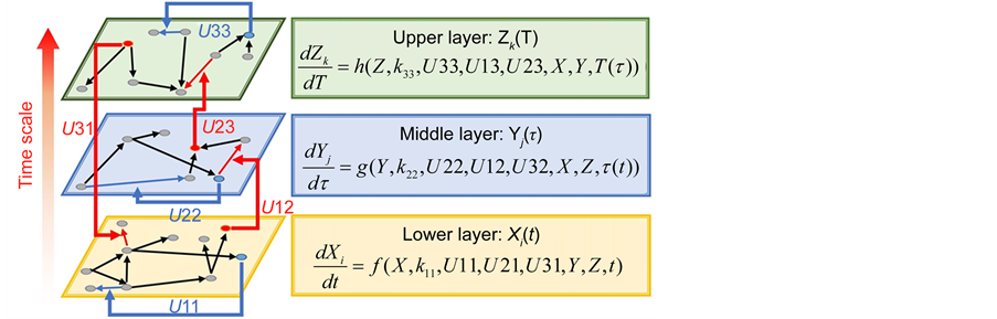
Figure 1. Overview of the multi-time-scale model; This model has three layers and has reactions across layers. The parameters  indicate concentrations;
  indicates the control variables from layer x to layer y;
  indicates the matrix of rate constants in layer n.
significant increases in computational demands (time stiff problem) [17] [18] [19] . Numerous implicit methods such as the Radau method [19] and Gear method [20] have been proposed as candidate solutions to the time stiff problem. These methods generate numerical solutions based on calculation sensitivities and stabilities of components in 1 layer. Furthermore, the numerical solutions of these methods are calculated using non-linear simultaneous equations with n unknowns based on n components in the model. In calculating multi-time-scale model using the implicit method, larger time step sizes than those for the smallest time-scale layer can be applied to numerical calculations of all layers because the calculation stability of the implicit method is very high. However, because multi-time-scale models comprise large numbers of components, non-linear simultaneous equations that are calculated using implicit methods become very large. Specifically, although implicit methods suppress increases in computational loads due to excessive reductions in adaptive step sizes, significant increases in volumes of numerical calculations for non-linear simultaneous equations cause failure to eliminate the time stiff problem. Parallel computing with reduced computational cost has been applied to numerical calculations of multi-time-scale models [21] [22] [23] . In contrast, contributions of parallel computing have been limited because analyses of dynamic behaviors of biological systems include numerous sequential calculations. These observations imply that the efficiency of numerical calculations in multi-time-scale models is highly dependent on reduced computational loads. Therefore, application of suitable step sizes to numerical calculations for each time scale layer will likely reduce computational loads significantly. Currently, few methods are available for determining suitable step sizes for numerical calculations of each layer in multi-time-scale models with interactions among layers, and solutions to this problem are essential for practical applications of multi-time-scale models to biological systems.
In this study, we developed a method for dynamically determining appropriate step sizes for the largest time-scale layer based on state changes of the smallest time-scale layer in numerical analysis of multi-time-scale models with interactions among layers. Subsequently, we proposed a numerical method for reducing computational loads of multi-time-scale models (proposed method) and verified the effectiveness of the proposed method using the follow steps:
1) Construction of multi-time-scale model (benchmark model) with interactions among layers that are universally observed in biological systems;
2) Numerical calculation of benchmark models using the conventional method (Control);
3) Numerical calculation of a benchmark model using the proposed method;
4) Comparison of computational loads for proposed and conventional methods;
5) Comparison of numerical solutions for proposed and conventional methods;
6) Discussion of the validity of the proposed method.
Using these procedures, we demonstrated the utility of the proposed method for improving computational efficiency without increasing computational costs of multi- time-scale models with interactions among layers. By reducing computational loads, the proposed method enhances the feasibility of mathematical analyses and accommodates greater scales of mathematical models, representing a significant contribution to systems biology methods.
2. Material and Methods
2.1. Benchmark Models with Multi-Time-Scales
To design and develop a method that is suitable for multi-time-scale models, we constructed 2 benchmark models (model A and model B) with the time stiff problem (Figure 2) and evaluated the calculation performance of the proposed method. The time stiff problem occurred due to differences in time-scales of each layer by interactions among layers. Thus, these benchmark models satisfied the following conditions: 1) Models included interactions across layers; 2) Models had different time-scales of each layer. Models A and B comprised lower, middle, and upper layers with time scales of seconds, minutes, and hours, respectively. Model A contained inhibition effects such as suppressed expression of anabolic enzymes by metabolic products [24] and negative control of gene expression by the lac repressor protein [25] , and these inhibition effects from upper to lower layers induced the time stiff problem with differences in time- scales of each layer caused by the largest time-scale layer (Figure 2(a)). Model B contained activation effects such as the transcriptional control by RNA polymerase [26] and the control of metabolic flux by enzymes [27] , and these activation effects from lower to upper layers induced the time stiff problem with differences in time-scales of each layer caused by the smallest time-scale layer (Figure 2(b)). Furthermore, these effects of activation and inhibition were expressed using the Hill equation [28] , which empirically explains cooperative effects of oxygen binding to hemoglobin. Equations (1)-(9) show mass balance equations of model A as follows:
 (1)
(1)

Figure 2. Case studies of multi-time-scale models; We verified the utility of the proposed method using two case studies. Both models have three layers with 60 time differences in time-scale order and were constructed using the Hill equation.
 (2)
(2)
 (3)
(3)
 (4)
(4)
 (5)
(5)
 (6)
(6)
 (7)
(7)
 (8)
(8)
 (9)
(9)
Here, Equations (1)-(3), (4)-(6), and (7)-(9) show magnitudes of change in lower, middle, and upper layers of model A, respectively. Table 1 shows kinetic parameters of Equations (1)-(9), and Equations (10)-(18) show mass balance equations of model B as follows:

Table 1.Constants and parameters in model A.
 (10)
(10)
 (11)
(11)
 (12)
(12)
 (13)
(13)
 (14)
(14)
 (15)
(15)
 (16)
(16)
 (17)
(17)
 (18)
(18)
Here, Equations (10)-(12), (13)-(15), and (16)-(18) show magnitudes of change in lower, middle, and upper layers of model B. Table 2 shows kinetic parameters of Equations (10)-(18). Normally, the time stiff problem occurs due to differences in time- scales of each component by dynamically changing reaction rates  in model A and B. In this paper, reaction rates were constant in entire time, to focus on the time difference between layers.
2.2. Numerical Solutions of the Benchmark Model Based on the Conventional Method
We obtained numerical solutions of benchmark models (Model A, Model B) shown in Figure 2 using the explicit 4 stage 4th-order Runge-Kutta method [29] as the conventional method. The simulation time was set at 36000 s because the dynamic behavior of the upper layer reached steady state at this time. The adaptive time step size  of the conventional method was set to 1.00E−03 s. Figures 3(a)-(c) and Figures 3(d)-(f) show time-dependent changes of component concentrations in models A and B, respectively. Moreover, Figure 3(a) and Figure 3(d), Figure 3(b) and Figure 3(e), and Figures 3(c) and Figure 3(f) show time-dependent changes in component concentrations for simulation times of 0 - 36,000 s (0 - 10 h), 0 - 600 s (0 - 10 min), and 0 - 10 s, respectively. Thus, dynamic behaviors of dependent variables of lower, middle, and

Table 2. Constants and parameters in model B.
upper layers were observed in time-scales of seconds, minutes, and hours, respectively. To verify calculation performance of the proposed method, we defined the results of these calculations as controls.
2.3. Design and Development of Proposed Method
In numerical calculations of the conventional method in multi-time-scale models, the adaptive time step size of the smallest time-scale layer (lower layer) was adopted in calculations for all layers. Hence, numbers of calculation steps of middle and upper layers were equal to that of the lower layer in the conventional method. Here we defined the process of calculating the concentration  of component S at the time
  from the concentration
  of component S at time t as 1 unit of the calculation (1 step), and
  was the adaptive time step size. Adaptive time step sizes of middle and upper layers in the conventional method were generally much smaller than suitable for these layers. Use of optimal step sizes for middle and upper layers in numerical calculations reduced the numbers of calculation steps for middle and upper layers. Therefore, we developed effective numerical calculation algorithms (proposed method) that optimally controlled adaptive time step sizes for each layer based on variations of differential component values.
The proposed method comprised ahead, backward, and cumulative algorithms. Ahead and cumulative algorithms reduced the numbers of calculation steps, whereas the backward algorithm ensured calculation accuracy. Initially, the ahead algorithm adopted the arbitrary conventional method for the calculation of the smallest time-scale layer (lower layer) and implemented the iterative numerical integration in the interval
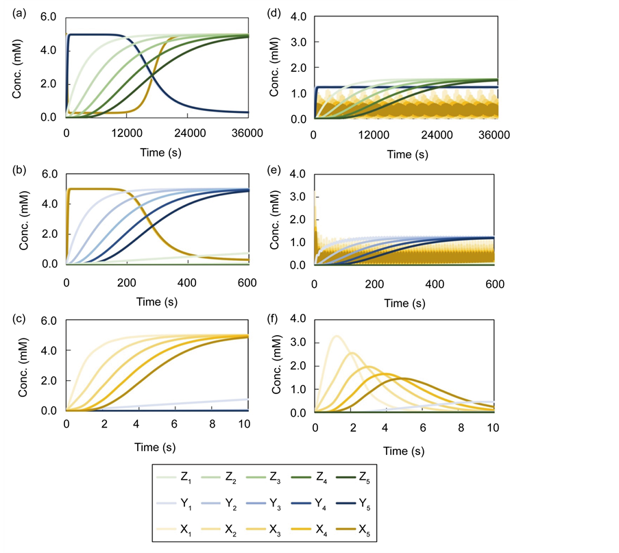
Figure 3. Time course of numerical solutions by the conventional method; The calculation step size dt of the conventional method was set to 1.00E−03 s. (a), (b), and (c) show results of the models A, (d), and (e), and (f) shows the result of model B. Simulation times of (a) and (d) were set to 36,000 s (10 h), those of (b) and (e) were set to 600 s (10 min), and those of (c) and (f) were set to 10 s.
of the arbitrary number of the  step, which was set to a predetermined calculation interval. Secondly, the backward algorithm was used to define a predetermined calculation interval in which the differential value was less than a certain value according to the determined calculation interval. Here, the adaptive time step size of the middle layer and the representative value for the lower layer were set to determine the calculation interval and its average integral value of the numerical solution for the lower layer. Subsequently, the cumulative algorithm was used to calculate the dynamics of the 1st step of the middle layer using these values. The proposed method repeated these 3 algorithms until the numerical solution of the upper layer was achieved. Thus, the adaptive time step sizes of middle and upper layers of the proposed method were much larger than those of the conventional method. Moreover, calculation steps of the proposed method were fewer than those of the conventional method, reflecting differing step sizes of proposed and conventional methods. In addition, adaptive time step sizes of middle and upper layers of the proposed method were controlled by the backward algorithm to maintain calculation accuracy. Accordingly, the computational volume of the proposed method was less than that of the conventional method and the calculation accuracies of proposed and conventional methods were comparable. Numerical calculations of the proposed method in the multi-time-scale models comprising the 3 layers of models A and B are described by Equations (19)-(21), which are mass balance equations and targets of the proposed method as follows:
 (19)
(19)
 (20)
(20)
 (21)
(21)
Equations (22) and (23) describe initial conditions as follows:
 (22)
(22)
 (23)
(23)
Here, the parameters  indicate concentration of components
  identified in each layer
  of lower, middle and upper layer.
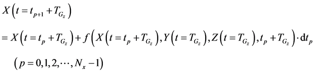
2.3.1. Ahead Algorithm
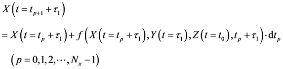
Initially, numbers of predetermined calculation steps  were set to 60 (Table 3). In the ahead algorithm, the arbitrary conventional method was adopted (Euler method [29] , Runge-Kutta method [29] , Runge-Kutta-Fehlberg method [30] etc.) with the numerical calculation of the smallest time-scale layer (lower layer), and the iterative numerical integration in the interval of the number of
  steps (predetermined calculation interval) was implemented. The numerical calculation from the initial state to the
  step was explicitly calculated based on Equations (24) and (25) as
Table 3. Parameters of the proposed method.
follows:
 (24)
(24)
 (25)
(25)
Here,  indicates the adaptive time step size per step in the lower layer, equations for middle and upper layers were shown in Equation (36) and (46), respectively.
2.3.2. Backward Algorithm
The backward algorithm was used to explore the predetermined calculation interval in which the differential value was less than a certain value according to the determined calculation interval. Here, the number of calculation steps was set to the number of determined calculation steps . Consequently, the backward algorithm could be used to monitor magnitudes of change in the numerical solution of dependent variables in the predetermined calculation interval. Subsequently, the backward algorithm narrowed the determined calculation interval for large changes in numerical solutions of the dependent variable in the predetermined calculation interval and widened that when changes were small. To measure magnitudes of change of all components in the layer, we compared the final differential value
  of each component at the time
  with the average integral value
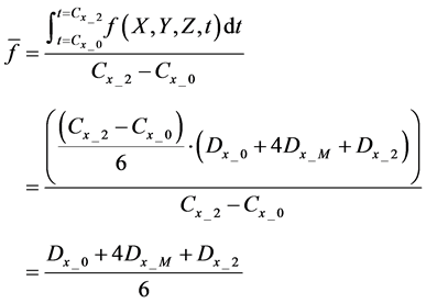
  of the differential value in the predetermined calculation interval using Equation (26) as follows:
 (26)
(26)
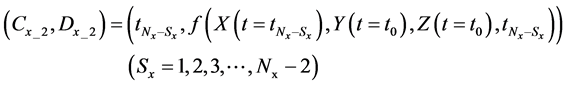
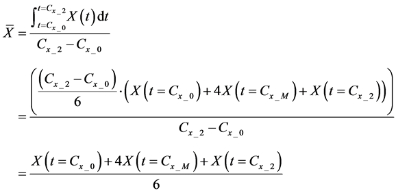
Here, E is evaluation value of each component in the predetermined calculation interval and this evaluation value shows the magnitude of change in the differential value of each component during the predetermined calculation interval. Using Simpson’s numerical integration method [29] to the coordinate points  of time and the differential value, we determined the average integral value
  of the differential value in the predetermined calculation interval. Equations (27)-(29) show the coordinate points
  of time and the differential value as follows:
 (27)
(27)
 (28)
(28)
 (29)
(29)
We obtained differential values  at the midpoint of the predetermined calculation interval
  using the Lagrange interpolation [29] as shown in Equations (30) and (31) as follows:
 (30)
(30)
 (31)
(31)
The average integral value  was calculated using the coordinate points
  and the differential value
  (Equation (32)) as follows:
 (32)
(32)
Evaluation value E (Equation (26)) was calculated as the average integral value  and the differential value
 . We determined the dependent variable of the lower layer when evaluation value E of all components in the lower layer were less than or equal to the threshold value (α) (E £ α). However, we updated the coordinate points
  to Equation (33) and calculated the
 ,
,  and evaluation value E when at least one of E were greater than the threshold value (α) (E > α) as follows:
 (33)
(33)
Thereafter, we sequentially increased the number of discarded calculation steps  until E of all components in the lower layer were less than or equal to the threshold value (α) (E £ α) and determined the dependent variable of the lower layer. The number of determined calculation steps
  was set to
  when the all evaluation values E were less than or equal to the threshold value (α) (Equation (34)) as follows:
 (34)
(34)
If E was more than the threshold value (α) at , we set it to
 . Equation (35) shows the coordinate points
  after the number of determined calculation steps
  was decided as follows:
 (35)
(35)
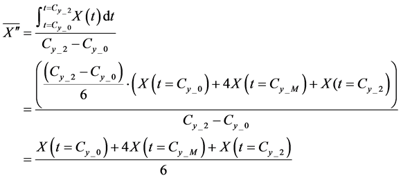
2.3.3. Cumulative Algorithm
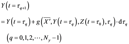
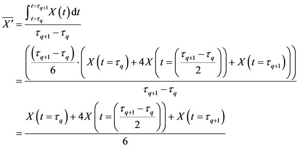
After determining the calculation interval of the lower layer with the backward algorithm, the cumulative algorithm was used to implement the numerical calculation of the 1st step in the middle layer using Equations (36)-(39) as follows:
 (36)
(36)
 (37)
(37)
 (38)
(38)
 (39)
(39)
Here,  was equal to the interval from time
  to time
  and
and  was the time-averaged concentration of the numerical solution of the lower layer in the interval from time
  to time
 . In addition,
  was calculated using Lagrange interpolation [29] . We applied the conventional method shown in the ahead algorithm to the numerical calculation of the middle layer.
2.3.4. Integration of Whole Algorithms
Calculations of these algorithms gave numerical solutions of lower and middle layers at time . Subsequently, the numerical solution of the concentration of the component in the interval from the
  step to the
  step in the lower layer (the predetermined calculation interval) was calculated using the ahead algorithm with the values
  and
and  as shown in Equation (40) as follows:
 (40)
(40)
Thereafter, the backward algorithm was used to define the number of determined calculation steps  and the number of discarded calculation steps
  in this predetermined calculation interval, and the cumulative algorithm was used to calculate
  of the middle layer. We repeated the procedures in Equations (26)-(40), and the numerical solution of the component concentration of the middle layer was calculated until the
  step (the predetermined calculation interval in the middle layer) using the following Equations (41) and (42):
 (41)
(41)
 (42)
(42)
Here,  denotes the time-averaged concentration of the numerical solution of the lower layer in the interval from time
  to
to . The number of determined calculation steps
  was then decided and the number of discarded calculation steps
  in middle layer was generated using the backward algorithm. Equations (43)-(45) show the coordinate points of the differential value and the time of the middle layer that is necessary for the corresponding calculation of E (Equation (26)) as follows:
 (43)
(43)
 (44)
(44)
 (45)
(45)
The cumulative algorithm was used to implement the calculation of the 1st step of the upper layer with numerical solutions of lower and middle layers using Equations (46)-(50) as follows:
 (46)
(46)
 (47)
(47)
 (48)
(48)
 (49)
(49)
 (50)
(50)
Here,  was equal to the interval from the time
  to the time
 , and
, and  was the corresponding time-averaged concentration of the numerical solution of the lower layer.
  was the time-averaged concentration of the numerical solution of the middle layer in the same time interval and
  and
and  were calculated using Lagrange interpolation [29] . The numerical calculation of the upper layer shown in Equation (46) applied the same conventional method in the case of the ahead algorithm (Equation (24)). Subsequently, we repeated Equations (26)-(50) and found the numerical solution from
  to
to  of the dependent variable in the upper layer. Finally, the backward algorithm was used to define the number of determined calculation steps
  and the number of discarded calculation steps
  in the upper layer. After completion of upper layer calculations, we calculated iterative numerical integrations in the interval of
  steps of the lower layer using the values
 ,
,  and
and  in Equation (51) as follows:
 (51)
(51)
Iterative calculations of component concentrations of all layers were calculated using Equations (26)-(51).
2.3.5. Control of Numbers of Predetermined Calculation Steps
Numbers of predetermined calculation steps  indicated numbers of calculations with the ahead algorithm. When numbers of predetermined calculation steps
  were excessively large, the backward algorithm discarded the calculation obtained by the ahead algorithm to maintain calculation accuracy. Therefore, the number of predetermined calculation steps
  was closely related to the calculation efficiency of the proposed method, and the number of predetermined calculation steps
  was dynamically changed based on the number of determined calculation steps as shown in Equation (52) as follows:
 (52)
(52)
Here,  were increments of the number of predetermined calculation steps
 . Accordingly, Equation (52) implicitly controlled the number of predetermined calculation steps of each layer according to the rate of change of the dependent variable.
2.4. Evaluation of Calculation Accuracy
The calculation accuracy of the proposed method was evaluated using Equations (53) and (54). Firstly, we evaluated calculation accuracy according to the consistency of the numerical solution using Equation (53) as follows:
 (53)
(53)
where  and
and  were corresponding to the numerical solution of specific
  in the layer of interest using the proposed and conventional method, respectively. The num represented the number of components in the layer of interest. The right side of Equation (53) was the average of proportion of the numerical solution from the proposed method
  to that of the conventional method
 . Secondly, we evaluated local calculation accuracy according to the standard deviation of the value between the numerical solution of the proposed method and that of the conventional method using Equation (54) as follows:
 (54)
(54)
Hence, calculation accuracy was evaluated according to  and
and .
.
3. Results
In the multi-time-scale models (Model A, Model B) shown in Figure 2, we compared numerical solutions of the proposed method with those of the conventional method. In the conventional method, we adopted the explicit 4 stage 4th-order Runge-Kutta method [29] for numerical calculations of all layers. However, the numerical calculation of the lower layer of the proposed method allowed application of the arbitrary method for ordinary differential equations. We also adopted the explicit 4 stage 4th-order Runge- Kutta method [29] for the numerical calculations of the lower layer of the proposed method. Table 1 and Table 2 show kinetic parameters of models A and B, respectively, and the simulation time was set to 36000 s because the dynamic behavior of the upper layer reached steady state at this time. The step size dt of the adaptive time of the explicit 4 stage 4th-order Runge-Kutta method [29] was used in the proposed method and the conventional method, and was set to 1.00E−03 s.
3.1. Case Study 1
As shown in Figure 2(a), model A comprises 18 components and has inhibition effects from upper to middle layers and from middle to lower layers. We compared numerical solutions of the proposed and conventional methods in model A and verified the utility of the proposed method in the multi-time-scale model in terms of calculation efficiency and accuracy. Table 3 shows parameters of initial numbers of predetermined calculation steps  and parameters of control variables for numbers of predetermined calculation steps
  of the proposed method. The threshold value (α) of the evaluation value E of the backward algorithm was set to 1.00E−03, 5.00E−04, and 1.00E−04.
3.1.1. Calculation Efficiency of the Proposed Method in Numerical Analyses of Model A
In numerical analyses of model A, the calculation efficiency of the proposed method was compared with that of the conventional method. Figures 4(a)-(c) show time- dependent changes in numbers of accumulated calculation steps for each layer in model A. Here, numbers of accumulated calculation steps for lower, middle, and upper layers were equal to the sum of 
 ,
, 
 and
and 
 within the entire simulation time for model A. We applied the same method to the numerical calculation for the lower layer of the proposed and conventional methods. Hence, numbers of accumulated calculation steps for the lower layer of the proposed method was equal to that of the conventional method (Figure 4(c)). Furthermore, we compared numbers of accumulated calculation steps in middle and upper layers of model A (Figure 4(a) and Figure 4(b)). Accumulated calculation steps in middle and upper layers of the proposed method at 36,000 s (Table 4) were far fewer than those of the conventional method in middle and upper layers of model A. Moreover, the threshold value (α) of the evaluation value E and the number of accumulated calculation steps of the proposed method in middle and upper layers were negatively correlated. Figure 4(d) shows the sum of calculation steps that were discarded by the backward algorithm, which ensured calculation accuracy. In these analyses, the sum of discarded calculation steps was equal to
  within the entire simulation time for model A. Moreover, regardless of the threshold value (α), destruction of the calculation by the backward algorithm occurred during the early stages of the simulation. In addition, destruction of calculations had occurred at 12,000 s when the threshold value (α) was 1.00E−3 or 5.00E−04. Figure 4(e) shows time-dependent changes in the sum of accumulated calculation steps for all layers of model A. The proposed method included the
Table 4. Calculation efficiency of the proposed method in middle and upper layers of model A at 36000 s.
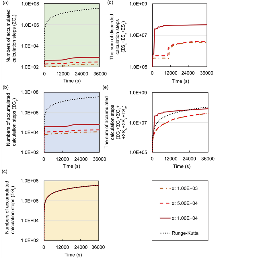
Figure 4. Comparisons of numbers of accumulated calculation steps for the proposed and conventional methods in model A; The calculation step size  was set at 1.00E−03 s. The threshold value (α) of the evaluation value E of the backward algorithm was set at 1.00E−03, 5.00E−04, and 1.00E−04. (a), (b), and (c) show the sum of numbers of accumulated calculation steps for lower, middle, and upper layers in model A
 . (d) shows the sum of calculation steps that were discarded by the backward algorithm in model A
 . (e) shows the sum of accumulated calculation steps of all layers in model A
  .
.
sum of calculation step that were discarded by the backward algorithm as
 . Accumulated calculation steps of the pro- posed method for all layers of model A at 36000 s are shown in Table 5 as a proportion of those for the conventional method. Because numbers of accumulated calculation steps of the proposed method in middle and upper layers (decreased numbers of calcu-
Table 5. Calculation efficiency of the proposed method in all layers of model A at 36000 s.
lation steps) were greater than those that were discarded by the backward algorithm (increased numbers of calculation steps), which was dependent on the threshold value (α), the sum of accumulated calculation steps for all layers of the proposed method was reduced.
3.1.2. Calculation Accuracy of Proposed Method in Numerical Analysis of Model A
The numerical solution of the proposed method was compared with that of the conventional method in model A. Figures 5(a)-(c) show time-dependent changes of the evaluation value  (Equation (53)), which represents consistency of the numerical solution. Figures 5(d)-(f) show time-dependent changes of the evaluation value
  (Equation (54)), which represents local calculation accuracy. In any layer,
  was within the range of 0.95 - 1.05 and
  was 0.01 or less at all times. Moreover,
  was asymptotic to 1.0 with decreases in thresholds (α) of the evaluation value E in all layers. Therefore, the calculation accuracy of the proposed method was almost the same as that of the conventional method in numerical analyses of model A.
3.2. Case Study 2
As shown in Figure 2(b), model B comprised 18 components and had activation effects from lower to middle layers and from middle to upper layers. In addition, the effect of negative feedback in the lower layer led to oscillating dynamics in model B. In the pre- sent study, we compared numerical solutions of the proposed and conventional methods in model B and verified the utility of the proposed method in the multi- time-scale model in terms of calculation efficiencies and accuracies. Table 3 shows parameters of initial numbers of predetermined calculation steps  and parameters of control variables for numbers of predetermined calculation steps
  of the proposed method. Threshold values (α) of the evaluation value E of the backward algorithm were set at 1.00E−01, 5.00E−02, and 1.00E−02.
3.2.1. Calculation Efficiency of the Proposed Method in Numerical Analyses of Model B
In numerical analysis of model B, the calculation efficiency of the proposed method was compared with that of the conventional method. Figures 6(a)-(c) show time-depen- dent changes in numbers of accumulated calculation steps for each layer of model B.

Figure 5. Comparison of calculation accuracies of the proposed and conventional methods in model A; Vertical axes of (a), (b), and (c) show  (Equation (53)). Vertical axes of (d), (e), and (f) show
  (Equation (54)). The threshold value (α) of the evaluation value E of the back- ward algorithm was set at 1.00E−03, 5.00E−04, and 1.00E−04.
Here, numbers of accumulated calculation steps of lower, middle, and upper layers were equal to sums of 
 ,
, 
 and
and 
 , respectively,
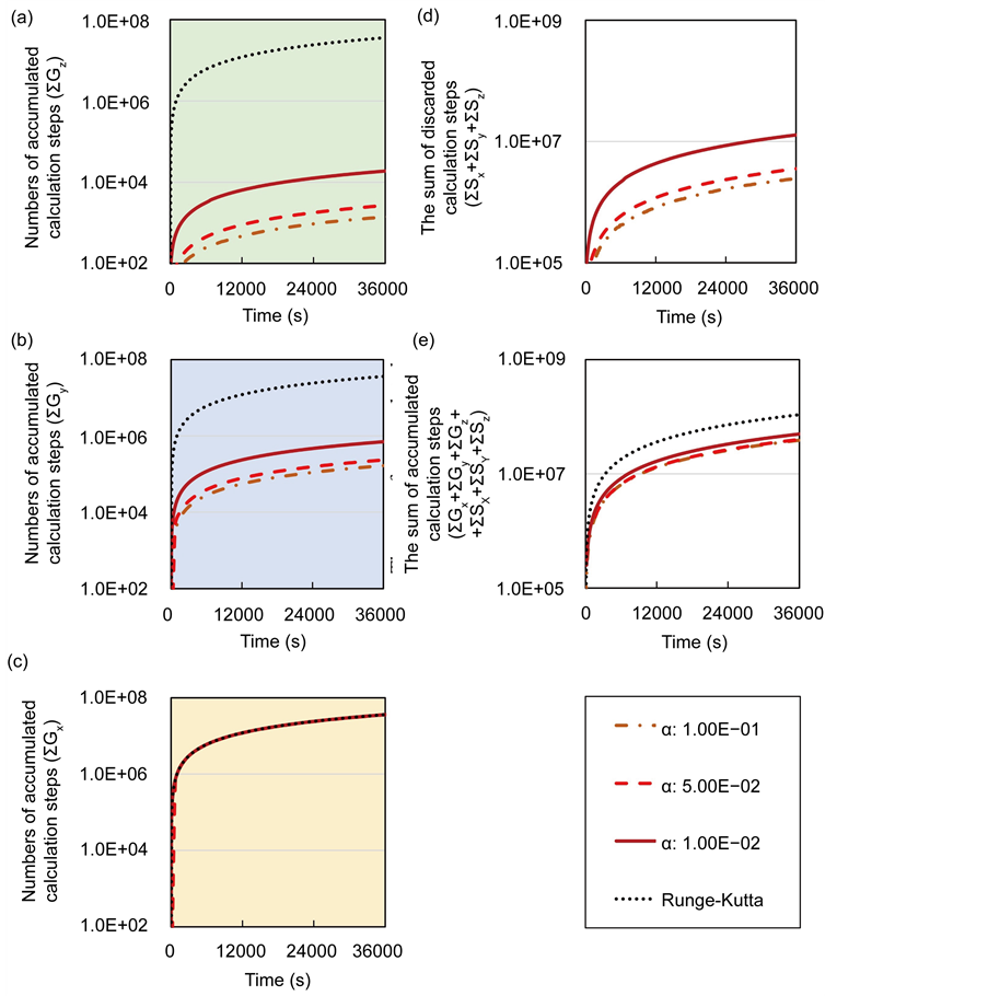
Figure 6. Comparison of numbers of accumulated calculation steps for proposed and conventional methods in model B; The calculation step size dt was set at 1.00E−03. The threshold value (α) of the evaluation value E for the backward algorithm was set at 1.00E−01, 5.00E−02, and 1.00E−02. (a), (b), and (c) show the sum of accumulated calculation steps for lower, middle, and upper layers in model B . (d) shows the sum of calculation steps that were discarded by the backward algorithm in model B
 . (e) shows the sum of accumulated calculation steps for all layers in model B
  .
.
within the entire simulation time of model B. Differences between numbers of accumulated calculation steps in the lower layer of the proposed and conventional methods are not demonstrated (Figure 6(c)) as well as in case study 1. However, in further analyses we compared numbers of accumulated calculation steps in middle and upper layers of model B (Figure 6(a) and Figure 6(b)). Table 6 shows numbers of accumulated calculation steps in middle and upper layers of the proposed method at 36000 s in model B relative to those of the conventional method. Numbers of accumulated calculation steps for the proposed method were far fewer than those of conventional method in middle and upper layers of model B. Moreover, threshold values (α) of E from the backward algorithm were negatively correlated with numbers of accumulated calculation steps of the proposed method in middle and upper layers. Figure 6(d) shows the sum of calculation steps that were discarded by the backward algorithm, which was used to ensure calculation accuracy. In these analyses, the sum of discarded calculation steps was equal to  within the entire simulation time for model B. In case study 2, the calculation was discarded at a constant rate with time. Figure 6(e) shows time-dependent changes of the sum of accumulated calculation steps for all layers in model B. The proposed method included the sum of calculation steps that were discarded by the backward algorithm as
 . Table 7 shows the sum of accumulated calculation steps for all layers of proposed method at 36000 s in model B as a proportion of that for the conventional method. In case study 2, decreases in numbers of accumulated calculation steps in middle and upper layers of the proposed method were greater than the increases in numbers of calculation steps that were discarded by the backward algorithm, which was dependent on the threshold value (α). Thus, the sum of accumulated calculation steps of all layers of the proposed method was reduced.
Table 6. Calculation efficiency of the proposed method in middle and upper layers of model B at 36,000 s.
Table 7. Calculation efficiency of the proposed method in all layers of model B at 36,000 s.
3.2.2. Calculation Accuracy of the Proposed Method for Numerical Analysis of Model B
The numerical solution of proposed method was compared with that of the conventional method in model B. Figures 7(a)-(c) show time-dependent changes in the evaluation value  (Equation (53)), which represents consistency of the numerical solution, and Figures 7(d)-(f) show time-dependent changes of the evaluation value
  (Equation (54)), which represents local calculation accuracy. In any layer,
  was within the range of 0.99 - 1.01, and
  was 0.01 or less at all times. Therefore, the calculation accuracy of the proposed method was almost the same as that of the conventional method in numerical analyses of model B.
4. Discussion
The advent of high-throughput experimental devices that can accommodate large numbers of samples has allowed simultaneous computation of comprehensive data pertaining to genome, transcriptome, proteome, and metabolome analyses [1] [2] [3] [4] [5] . Consequently, the momentum of theoretical analyses of biological systems that use multi-time-scale models is growing [13] [14] [15] [16] (Figure 1). In theoretical analyses of multi-time-scale models with reactions between layers, the time stiff problem [17] [18] [19] occurs due to differences in time-scales of each layer, leading to significant increases in computation times. In particular, the time stiff problem significantly influences the efficiency of numerical optimizations of system identifications and analyses. Optimization methods are generally used to search for optimum solutions using repeated calculations with varying kinetic parameters for different strategies. For example, system identification by the Real-coded Genetic Algorithm (AREX + JGG) required about 2.0E+06 calculation iterations to estimation parameter values for 112 elements [31] . Calculation times for numerical optimization are generated by multiplying numbers of calculations by the time taken for 1 calculation. Because the time taken for 1 calculation is greatly increased by time stiff problems, calculation times for numerical optimizations also increase linearly. Hence, solutions for the time stiff problem will likely contribute to the efficiency of numerical optimizations. The time stiff problem also occurs in theoretical analyses of natural phenomena, such as the movements of the local clouds and typhoons in simulations of weather conditions [32] and motions and binding of compounds in simulations of chemical reactions [33] . Hence, solutions to the time stiff problem are applicable to varied mathematical analyses, including those of biological systems. In the present conventional method, the time stiff problem remained because the calculation of all layers was implemented by adaptive time step sizes of the smallest time-scale layer. Therefore, the present alternative method reduced computation times by controlling adaptive time step sizes for each layer based on variations of differential values of the components.
The proposed method comprised ahead, backward, and cumulative algorithms. Initially, the ahead algorithm was applied using the conventional method for calculating the smallest time-scale layer (lower layer), and iterative numerical integrations were
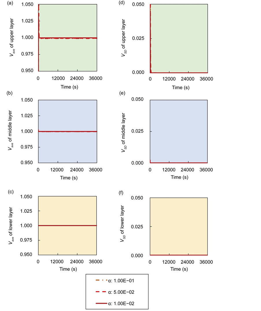
Figure 7. Comparison of calculation accuracies of the proposed and conventional methods in model B; Vertical axes of (a), (b), and (c) show  (Equation (53)). Vertical axes of (d), (e), and (f) show
  (Equation (54)). The threshold value (α) of the evaluation value E of the back- ward algorithm was set at 1.00E−03, 5.00E−04, and 1.00E−04.
performed in predetermined calculation intervals. In this study, we used the explicit 4 stage 4th-order Runge-Kutta method [29] to calculate the lower layer and then used the backward algorithm to determine the calculation interval according to the magnitude of change in the differential value during the predetermined calculation interval. Subsequently, the cumulative algorithm calculated the 1st step of the middle layer using the determined calculation interval of the lower layer and the time-averaged concentration in the determined calculation interval of the lower layer. The proposed method identified numerical solutions by repeating the three algorithms for the upper layer. In the conventional method, numbers of calculation steps for middle and upper layers were equal to that of the lower layer so that all layers were calculated according to the adaptive time step size of the lower layer. However, the adaptive time step size of middle and upper layers of the proposed method were much larger than those of the conventional method. In addition, the backward algorithm narrowed the calculation interval for large changes in the numerical solution of the predetermined calculation interval and widened that in the presence of small changes. Accordingly, the proposed method significantly reduced the number of calculation steps for middle and upper layers and maintained calculation accuracy of the backward algorithm. Most current high-speed calculation methods utilize parallel computer resources [21] [22] [23] , which are expedited by dividing the processing of calculations of 1 step between multiple central processing units. In contrast, the proposed method accelerates analyses by reducing numbers of calculation steps. Therefore, the proposed method does not compete with conventional high-speed methods, and can be used in conjunction with various high-speed calculation methods as a calculation module.
In the present study, we created multi-time-scale models as a benchmark (Figure 2) and verified the calculation performance of the proposed method. To this end, we investigated numbers of accumulated calculation steps for each layer of proposed and conventional methods. In case studies 1 and 2, numbers of accumulated calculation steps for the lower layer were comparable in proposed and conventional methods, whereas these were fewer for middle and upper layers of the proposed method than of the conventional method (Figures 4(a)-(c), Figures 6(a)-(c)). Therefore, calculations of middle and upper layers were performed using the proposed method with optimal adaptive time step sizes.
In further analyses, we discarded calculation steps to maintain calculation accuracy in backward algorithm. In case study 1, the sum of discarded calculation steps rapidly increased between the early stages of the simulation and 12,000 s (Figure 4(d)). Moreover, increasing numbers of discarded calculation steps during early stages of the simulation were greatly affected by initial setting values of , which are parameters of the proposed method. Accordingly, the ahead algorithm of the proposed method was used to calculate numerical solutions to initial setting values of
 , and the backward algorithm was used to discard calculations and maintain calculation accuracy. Therefore, the present backward algorithm significantly discarded significant numbers of calculations in the early stages of the simulation, because the initial setting values of
  were excessive. Moreover, increasing numbers of discarded calculation steps in the first 12000 s were greatly affected by variations of the dependent variable of model A (Figure 3). These variations reflected decreased inhibition effects of
  based on increases of
  and enhancements of the inhibitory effects of
 . To prevent the deterioration of calculation accuracy due to these variations, the backward algorithm was used to adjust the adaptive time step size for each layer to values that corresponded with magnitudes of change in numerical solutions of the dependent variable. Hence, the backward algorithm significantly discarded calculations by 12,000 s in case study 2. The sum of discarded calculation steps also increased linearly with time (Figure 6(d)). Because model B was of the oscillation system, destruction by the backward algorithm occurred in constant cycles. These analyses suggest that the backward algorithm facilitates calculation accuracy.
Numbers of accumulated calculation steps of all layers of proposed and conventional methods were computed for case studies 1 and 2, and decreases by the proposed method for middle and upper layers (Figure 4(a) and Figure 4(b), Figure 6(a) and Figure 6(b)) were greater than increases in those discarded by the calculation steps of the backward algorithm (Figure 4(d), Figure 6(d)). Hence, because reductions in computational volumes by the proposed method were more numerous than those required to maintain calculation accuracy, the proposed method achieved the calculation efficiency of the numerical calculation in case studies 1 and 2 (Figure 4(e), Figure 6(e)).
In comparisons of calculation accuracies of proposed and conventional methods, that of the proposed method was controlled by the threshold (α) of the evaluation value E. The calculation interval that was determined by the backward algorithm was asymptotic to predetermined calculation intervals with the increase of the threshold (α). Time step sizes of middle and upper layers also became larger. Moreover, the numerical solution of the upper layer was reflected in lower and middle layers after 1 step of upper layer calculations. Thus, this reflection time was significantly delayed with excessive step sizes of the upper layer in the presence of high threshold (α) values. This delay caused calculation error in the numerical solution of the proposed method. Hence, threshold (α) values of models that contains reactions from upper to lower layers such as case study 1 need to be smaller than that in the model for case study 2. In this study, threshold (α) values of case study 1 (1.00E−03, 5.00E−04, and 1.00E−04) were set smaller than that of case study 2 (1.00E−01, 5.00E−02, 1.00E−02). Accordingly, at threshold (α) values of 1.00E−03 or 5.00E−04, calculation errors occurred in middle and upper layers for case study 1. However, at threshold (α) < 1.00E−04, calculation errors were avoided. Therefore, in case studies 1 and 2, the calculation accuracy of the conventional method was maintained by the proposed method by setting the optimal threshold (α) value depending on the model (Figure 5, Figure 7).
5. Conclusion
In summary, in the present benchmark model, ahead and cumulative algorithms of the proposed method led to calculation efficiency of numerical calculations with adjustments of step sizes of each layer, and reduced the numbers of numerical calculations required for multi-time-scale models with the time stiff problem. Moreover, backward algorithms of the proposed method ensured calculation accuracy in the multi-time- scale model. Accordingly, we suggest that the proposed method is an efficient numerical method for multi-time-scale models.
Acknowledgements
This work was supported by Grant-in-Aid for Scientific Research on Innovative Areas 16H01700 and Grant-in-Aid for Challenging Exploratory Research16K12912.
Cite this paper
Motomura, Y., Hamada, H. and Okamoto, M. (2016) An Effective Numerical Calculation Method for Multi-Time-Scale Mathematical Models in Systems Biology. Applied Mathematics, 7, 2241-2268. http://dx.doi.org/10.4236/am.2016.717178
References
- 1. Castel, D., Pitaval, A., Debily, M.A. and Gidrol, X. (2006) Cell Microarrays in Drug Discovery. Drug Discovery Today, 11, 13-14.
https:/doi.org/10.1016/j.drudis.2006.05.015 - 2. Aebersold, R. and Mann, M. (2003) Mass Spectrometry-Based Proteomics. Nature, 13, 198-207.
https:/doi.org/10.1038/nature01511 - 3. Bleicher, K.H., Böhm, H.J., Müller, K. and Alanine, A.I. (2003) A Guide to Drug Discovery: Hit and Lead Generation: Beyond High-Throughput Screening. Nature Reviews Drug Discovery, 2, 369-378.
https:/doi.org/10.1038/nrd1086 - 4. Macarron, R., Banks, M.N., Bojanic, D., Burns, D.J., Cirovic, D.A., Garyantes, T., Green, D.V., Hertzberg, R.P., Janzen, W.P., Paslay, J.W., Schopfer, U. and Sittampalam, G.S. (2011) Impact of High-Throughput Screening in Biomedical Research. Nature Reviews Drug Discovery, 10, 188-195.
https:/doi.org/10.1038/nrd3368 - 5. Fischer, E., Zamboni, N. and Sauer, U. (2004) High-Throughput Metabolic Flux Analysis Based on Gas Chromatography-Mass Spectrometry Derived 13C Constraints. Analytical Biochemistry, 325, 308-316.
https:/doi.org/10.1016/j.ab.2003.10.036 - 6. Ge, H., Walhout, A.J. and Vidal, M. (2003) Integrating “Omic” Information: A Bridge Between Genomics and Systems Biology. Trends in Genetics, 19, 551-560.
https:/doi.org/10.1016/j.tig.2003.08.009 - 7. Altaf-Ul-Amin, M., Afendi, F.M., Kiboi, S.K. and Kanaya, S. (2014) Systems Biology in the Context of Big Data and Networks. BioMed Research International, 2014, Article ID: 428570.
https:/doi.org/10.1155/2014/428570 - 8. Hood, L. (2003) Leroy Hood Expounds the Principles, Practice and Future of Systems Biology. Drug Discovery Today, 8, 436-438.
https:/doi.org/10.1016/S1359-6446(03)02710-7 - 9. Kitano, H. (2002) Systems Biology: A Brief Overview. Science, 295, 1662-1664.
https:/doi.org/10.1126/science.1069492 - 10. Kitano, H. (2002) Computational Systems Biology. Nature, 420, 206-210.
https:/doi.org/10.1038/nature01254 - 11. Liu, E.T. (2005) Systems Biology, Integrative Biology, Predictive Biology. Cell, 121, 505-506.
https:/doi.org/10.1016/j.cell.2005.04.021 - 12. Papp, B., Notebaart, R.A. and Pál, C. (2011) Systems-Biology Approaches for Predicting Genomic Evolution. Nature Reviews Genetics, 12, 591-602.
https:/doi.org/10.1038/nrg3033 - 13. Yao, Z., Petschnigg, J., Ketteler, R. and Stagljar, I. (2015) Application Guide for Omics Approaches to Cell Signaling. Nature Chemical Biology, 11, 387-397.
https:/doi.org/10.1038/nchembio.1809 - 14. Bajikar, S.S. and Janes, K.A. (2012) Multiscale Models of Cell Signaling. Annals of Biomedical Engineering, 40, 2319-2327.
https:/doi.org/10.1007/s10439-012-0560-1 - 15. Helikar, T., Kochi, N., Kowal, B., Dimri, M., Naramura, M., Raja, S.M., Band, V., Band, H. and Rogers, J.A. (2013) A Comprehensive, Multi-Scale Dynamical Model of ErbB Receptor Signal Transduction in Human Mammary Epithelial Cells. PLoS ONE, 8, e61757.
https:/doi.org/10.1371/journal.pone.0061757 - 16. Stolarska, M.A., Kim, Y. and Othmer, H.G. (2009) Multi-Scale Models of Cell and Tissue Dynamics. Philosophical Transactions of the Royal Society, 367, 3525-3553.
https:/doi.org/10.1098/rsta.2009.0095 - 17. Curtiss, C.F. and Hirschfelder, J.O. (1952) Integration of Stiff Equations. Proceedings of the National Academy of Sciences of the United States of America, 38, 235-243.
https:/doi.org/10.1073/pnas.38.3.235 - 18. Sommeijer, B.P. (1993) Parallel-Iterated Runge-Kutta Methods for Stiff Ordinary Differential Equations. Journal of Computational and Applied Mathematics, 45, 151-168.
https:/doi.org/10.1016/0377-0427(93)90271-C - 19. Hairer, E. and Wanner, G. (1999) Stiff Differential Equations Solved by Radau Methods. Journal of Computational and Applied Mathematics, 111, 93-111.
https:/doi.org/10.1016/S0377-0427(99)00134-X - 20. Gear, C.W. (1971) Numerical Initial Value Problems in Ordinary Differential Equations. Prentice-Hall, Hoboken.
- 21. Gear, C.W. (1988) Parallel Methods for Ordinary Differential Equations. International Symposium on Vector and Parallel Processors for Scientific Computation, 25, 1-20.
https:/doi.org/10.1007/bf02575744 - 22. Bellen, A., Vermiglio, R. and Zennaro, M. (1990) Parallel ODE-Solvers with Stepsize Control. Journal of Computational and Applied Mathematics, 31, 277-293.
https:/doi.org/10.1016/0377-0427(90)90170-5 - 23. Pope, B.J., Fitch, B.G., Pitman, M.C., Rice, J.J. and Reumann, M. (2011) Performance of Hybrid Programming Models for Multiscale Cardiac Simulations: Preparing for Petascale Computation. IEEE Transactions on Biomedical Engineering, 58, 2965-2969.
https:/doi.org/10.1109/TBME.2011.2161580 - 24. Herrero, A., Muro-Pastor, A.M. and Flores, E. (2001) Nitrogen Control in Cyanobacteria. Journal of Bacteriology, 183, 411-425.
https:/doi.org/10.1128/JB.183.2.411-425.2001 - 25. Lewis, M., Chang, G., Horton, N.C., Kercher, M.A., Pace, H.C., Schumacher, M.A., Brennan, R.G. and Lu, P. (1996) Crystal Structure of the Lactose Operon Repressor and Its Complexes with DNA and Inducer. Science, 271, 1247-1254.
https:/doi.org/10.1126/science.271.5253.1247 - 26. Gruber, T.M. and Gross, C.A. (2003) Multiple Sigma Subunits and the Partitioning of Bacterial Transcription Space. Annual Review of Microbiology, 57, 441-466.
https:/doi.org/10.1146/annurev.micro.57.030502.090913 - 27. Suarez, R.K., Staples, J.F., Lighton, J.R.B. and West, T.G. (1997) Relationships between Enzymatic Flux Capacities and Metabolic Flux Rates: Nonequilibrium Reactions in Muscle Glycolysis. Proceedings of the National Academy of Sciences of the United States of America, 94, 7065-7069.
https:/doi.org/10.1073/pnas.94.13.7065 - 28. Goutelle, S., Maurin, M., Rougier, F., Barbaut, X., Bourguignon, L., Ducher, M. and Maire, P. (2008) The Hill Equation: A Review of Its Capabilities in Pharmacological Modeling. Fundamental & Clinical Pharmacology, 22, 633-648.
https:/doi.org/10.1111/j.1472-8206.2008.00633.x - 29. Press, W.H., Teukolsky, S.A., Vetterling, W.T. and Flannery, B.P. (2007) Numerical Recipes. 3rd Edition, Cambridge University Press, Cambridge.
- 30. Fehlberg, E. (1970) Klassische Runge-Kutta-Formeln vierter und niedrigerer Ordnung mit Schrittweiten-Kontrolle und ihre Anwendung auf Wärmeleitungsprobleme. Computing, 6, 61-71.
https:/doi.org/10.1007/BF02241732 - 31. Komori, A., Maki, Y., Nakatsui, M., Ono, I. and Okamoto, M. (2012) Efficient Numerical Optimization Algorithm Based on New Real-Coded Genetic Algorithm, AREX + JGG, and Application to the Inverse Problem in Systems Biology. Applied Mathematics, 3, 1463-1470.
https:/doi.org/10.4236/am.2012.330205 - 32. Arakawa, A. and Jung, J.H. (2011) Multiscale Modeling of the Moist-Convective Atmosphere—A Review. Atmospheric Research, 102, 263-285.
https:/doi.org/10.1016/j.atmosres.2011.08.009 - 33. Duarte, F., Amrein, B.A., Blaha-Nelson, D. and Kamerlin, S.C. (2015) Recent Advances in QM/MM Free Energy Calculations Using Reference Potentials. Biochimica et Biophysica Acta, 1850, 954-965.
https:/doi.org/10.1016/j.bbagen.2014.07.008