Applied Mathematics
Vol.06 No.12(2015), Article ID:61548,21 pages
10.4236/am.2015.612185
A Computational Study with Finite Element Method and Finite Difference Method for 2D Elliptic Partial Differential Equations
George Papanikos, Maria Ch. Gousidou-Koutita
School of Mathematics, Aristotle University, Thessaloniki, Greece

Copyright © 2015 by authors and Scientific Research Publishing Inc.
This work is licensed under the Creative Commons Attribution International License (CC BY).


Received 21 September 2015; accepted 27 November 2015; published 30 November 2015

ABSTRACT
In this paper, we consider two methods, the Second order Central Difference Method (SCDM) and the Finite Element Method (FEM) with P1 triangular elements, for solving two dimensional general linear Elliptic Partial Differential Equations (PDE) with mixed derivatives along with Dirichlet and Neumann boundary conditions. These two methods have almost the same accuracy from theoretical aspect with regular boundaries, but generally Finite Element Method produces better approximations when the boundaries are irregular. In order to investigate which method produces better results from numerical aspect, we apply these methods into specific examples with regular boundaries with constant step-size for both of them. The results which obtained confirm, in most of the cases, the theoretical results.
Keywords:
Finite Element Method, Finite Difference Method, Gauss Numerical Quadrature, Dirichlet Boundary Conditions, Neumann Boundary Conditions

1. Introduction
Finite Difference schemes and Finite Element Methods are widely used for solving partial differential equations [1] . Finite Element Methods are time consuming compared to finite difference schemes and are used mostly in problems where the boundaries are irregular. In particularly, it is difficult to approximate derivatives with finite difference methods when the boundaries are irregular. Moreover, Finite Element methods are more complicated than Finite Difference schemes because they use various numerical methods such as interpolation, numerical integration and numerical methods for solving large linear systems (see [2] - [6] ). Also the mathematically derivation of Finite Element Methods come from the theory of Hilbert Space, and Sobolev Spaces as well as from variational principles and the weighted residual method (see [5] -[12] ).
In this paper, we will describe the Second order Central Difference Scheme and the Finite Element Method for solving general second order elliptic partial differential equations with regular boundary conditions on a rectangular domain. In addition, for both of these methods, we consider the Dirichlet and Neumann Boundary conditions, along the four sides of the rectangular area. Also, we make a brief error analysis for Finite element method. Moreover, for the finite element method, we site two other important numerical methods which are important in order that the algorithm can be performed.
These methods are the bilinear interpolation over a linear Lagrange element, Gauss quadrature and contour Gauss Quadrature on a triangular area. Furthermore, these two schemes lead to a linear system which we have to solve. For the purpose of this paper, we solve the outcome systems with Gauss-Seidel method which is briefly discussed. In the last section, we contacted a numerical study with Matlab R2015a. We apply these methods into specific elliptical problems, in order to test which of these methods produce better approximations when the Dirichlet and Neumann boundary conditions are imposed. Our results show us that the accuracy of these two methods depends on the kind of the elliptical problem and the type of boundary conditions. In Section 2, we study the Second order Central Difference Scheme. In Section 3, we give the Finite Element Method, bilinear interpolation in P1, Gauss Quadrature, Finite Element algorithm and error analysis. In Section 4, we give some numerical results, in Section 5, we give the conclusions and finally in Section 6 we give the relevant references.
2. Second Order Central Difference Scheme
The second order general linear elliptic PDE of two variables x and y given as follow:
 (1)
(1)
with u defined on a rectangular domain
 , it holds
 . Also
 and
and 
Moreover in this paper two types of boundary conditions are considered:
 (Dirichlet Boundary Conditions).
 (Neumann Boundary Conditions).
The boundary
 and n is the normal vector along the boundaries.
We divide the rectangular domain Ω in a uniform Cartesian grid

where N , M are the numbers of grid points in x and y directions and

are the corresponding step sizes along the axes x and y. The discretize domain are shown in Figure 1.
Using now the central difference approximation we can approximate the partial derivatives of the relation (1) as follows:
 (2)
(2)
 (3)
(3)
 (4)
(4)
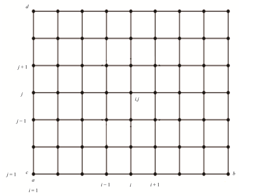
Figure 1. Discrete domain.
 (5)
(5)
 (6)
(6)
where
 are the truncation errors.
We now approximate the PDE (1) using the relations (2), (3), (4), (5), (6) and we obtain the second order central difference scheme:
 (7)
(7)
With truncation error .
.
The relation (7) can be written as a linear system:
 (8)
(8)
Dirichlet Boundary Conditions
The dimensions of the above linear system depends on the boundary conditions. More specific, if we have the Dirichlet Boundary Conditions:

then the dimensions of the matrix A, u and b are:
 for the vectors u, b and

for the matrix A. Moreover, the form of matrix A and the vector u are given by:
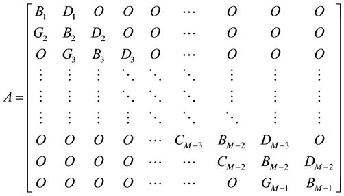
and

As we can see the matrix A is tri-diagonal block Matrix. These block matrices

are tri-diagonal as well of order

Neumann Boundary Conditions
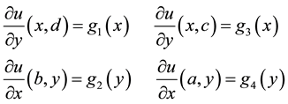
We approximate the Neumann boundary conditions in every side of the rectangular domain as follows
1st side (North side of the rectangular area)
 (9)
(9)
2nd side (East side of the rectangular area)
 (10)
(10)
3rd side (South side of the rectangular area)
 (11)
(11)
4th side (West side of the rectangular area)
 (12)
(12)
Using the relations (9), (10), (11), (12) the values
 which lies outside the rectangular domain can be eliminated when appeared in the linear system.
Thus the block tri-diagonal matrix A has dimensions
 and the vectors u, b are of
 order. The matrix A and the vector u are given below:
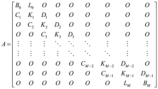
and

where
 are tri-diagonal matrices with dimensions
 .
.
In order to solve the linear system (8), we use the Gauss-Seidel method (GSM) (see [2] [3] ). An important property that the matrix A must have is to be strictly diagonally dominant in order the GCM to converge.
Theorem 1
If A is strictly diagonally dominant, then for any choice of
 , Gauss-Seidel method give sequence

that converge to the unique solution of
 .
.
The proof of theorem 1 can be found in [2] [3] .
3. Finite Element Method
In this section we consider an alternative form of the general linear PDE (1)
 (13)
(13)
where
 and
and
 .
.
With boundary conditions
 (Dirichlet Boundary Conditions).
 (Neumann Boundary Conditions).
And the boundary

In order to approximate the solution of (13) with FEM algorithm we must transform the PDE into its weak form and solve the following problem.
Find

 (14)
(14)
where

and

are bilinear and linear functionals as well.
It is sufficient now to consider that
 ,
,
 . Also we assume that
 and
and 
when the Neumann boundary Conditions are applied
 , else if we have only Dirichlet Boundary
conditions then the line integral is equal to zero.
The finite element method approximates the solution of the partial differential Equation (13) by minimizing the functional:
 (15)
(15)
where
 and
and
 . Also with D we denote
the weak derivatives of u. The spaces
 ,
,
 are Sobolev function spaces which also considered to be Hilbert spaces(see [7] -[9] ).
The uniqueness of the solution of weak form (14) depends on Lax-Milgram theorem along with trace theorem (see [7] ). In addition according to Rayleigh-Ritz theorem the solution of the problem (14) are reduced to minimization of the linear functional
 , (see [7] ).
The first step in order the FEM algorithm to be performed is the discretization of the rectangular domain
 by using Lagrange linear triangular elements.
We denote with Pk the set of all polynomials of degree
 in two variables [7] . For k = 1 we have the linear Lagrange triangle and

Also the triangulation of the rectangular area should have the below properties:
We assume that the triangular elements , are open and disjoint, where h is the maximum diameter of the triangle element.
The vertices of the triangles all call nodes, we use the letter V for vertices and E for nodes.
We also assume that there are no nodes in the interior sides of triangles.
3.1. Bilinear Interpolation in P1
Let as consider now the triangulation of the rectangular domain
 as we describe to a previous section. In every triangle Ti of the domain we interpolate the function u with the below linear polynomial:

with interpolation conditions:

in every vertex
 of a triangular element.
Thus it creates the below linear system with unknown coefficients a, b, c.

Solving the system we find the approximate polynomial of u

where
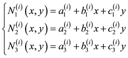
and
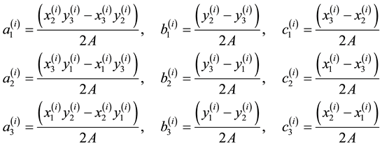
The function
 is the interpolation function or shape function and it has the following property:

3.2. Gauss Quadrature
An important step in order to implement the Finite Element algorithm is to compute numerically the double and line integrals which occurs in every triangular element (see [5] [12] ).
Gauss Quadrature in Canonical Triangle
As a canonical triangle we consider the triangle with vertices (0, 0), (0, 1) and (1, 0) and we denote
 . The approximation rule of the double integral in canonical triangle is given below:

Where ng is the number of Gauss integration points, wi are the weights and
 are the Gauss integration points.
The linear space Pκ is the space of all linear polynomial of two variables of order k
The following Table 1 gives the number of quadrature points for degrees 1 to 4 as given in Ref. [10] . It should be mentioned that for some N, the corresponding ng is not necessarily unique. (see [10] and references therein).
Gauss quadrature in general triangular element
Initially we transform the general triangle Τ into a canonical triangle using the linear basis functions:


Table 1. Quadrature points for degrees 1 to 4.
The variables x, y for the random triangle can be written as affine map of basis functions:

Also we have the Jacobian determinant of the transformation

Using the above relations we obtain the Gauss quadrature rule for the general triangular element:

with

is the area of the triangle.
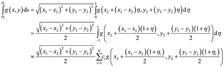
Contour quadrature rule
In the Finite Element Method when the Neumann boundary conditions are imposed it is essential to compute numerically the below Contour integral in general triangular area.

The basic idea is to transform the straight contour PiPj to an interval
 , and then the Gaussian quadrature for single variable function.
Using the basis functions we have the following relations in every side of the triangle
Along side 1 (P1P2) :

Along side 3: (P3P1):

Along side 2: (P2P3):
The error of the bilinear interpolation Gauss quadrature depend on the dimension of the polynomial subspace (see [11] ).
3.3. Finite Element Algorithm
The Finite element algorithm has the purpose to find the approximate solution of the problem (15) in a subspace of
 . We consider as subspace the
 of all piecewise linear polynomials with two variables polynomials of degree one. i.e.:

The index i represents the number of triangular elements which exist in the rectangular domain. The polynomials must be piecewise because the linear combination of them must form a continuous and integrable function with continuous first and second derivatives.
The existence and uniqueness of the approximate solution is ensured by the Lax-Milgram-Galerkin and Rayleight- Ritz theorems (see [1] [7] [8] ).
Firstly as we describe in a previous section, we have to triangulate the domain before the algorithm evaluated.
After that the algorithm seeks approximation of the solution of the form:

where
 is the linear combination of independent piecewise linear polynomials and
 are constants with m is the number of nodes. Actually, the polynomials
 corresponds to shape functions
 in every vertex of the triangles. Thus the approximate solution is the linear combination of all the independent interpolation functions multiplied with some constant
 . Some of these constants for example,
 are used to ensure that the Dirichlet boundary conditions if there are exist

are satisfied on
 and the remaining constants
 are used to minimize the functional
 .
.
Inserting the approximate solution
 for v into the functional
 and we have:
 (16)
(16)
Consider J as a function of
 . For minimum to occur we must have

Differentiating (16) gives

for each

 .This set of equations can be written as a linear system:
 (17)
(17)
where
 ,
,
 and
and
 are defined by

for each

 .
.

The choice of subspace
 for our approximation is important because can ensure us that the matrix A will be positive definite and band( [2] -[4] ). According to the previous analysis leads again to a linear system, which can be solved as we described in a previous section with Gauss-Seidel Method (see [2] -[4] ).
3.4. Error Analysis
Let us consider again the problem (14)
Find
 :
:
 (18)
(18)
The approximation of finite element of the problem (18) is given below:
Find
 :
:
 (19)
(19)
Cea’s lemma
The finite element approximation
 of the weak solution
 is the best fit to in the norm
 i.e:
i.e:

The error analysis of finite element method depend on the Cea’s lemma for elliptic boundary value problems. The proof can be found in [1] [7] .
Now we will present without proof the following statement [7] .
 (20)
(20)
where
 is positive constant dependent on the smoothness of the function u, h is the mesh size parameter and s is a positive real number, dependent on the smoothness of u and the degree of the piecewise polynomials comprising in
 . In our case we have the Lagrange linear elements so the degree of the piecewise polynomials is one. Combining, relations Cea’s lemma we shall be able to deduce that:
 (21)
(21)
The relation (21) gives a bound of the global error
 in terms of the size mesh parameter h . Such a bound on the global error is called priori error bound.
L2-norm
For proving an error estimate in L2-norm the regularity of the solution of (13) plays an essential role. By the Aubin-Nitsche duality argument the error estimate in L2 norm between u and its finite element approximation
 is
is . However this bound can be improved to
 , (see [1] [7] ).
4. Numerical Study
In this section we contact a numerical study using Matlab R2015a. For the purpose of this paper we cite representative examples of second order general elliptic partial differential equations in order to make comparisons between these two methods with various step-sizes and the mesh size parameters of finite element method. Thus in each example we present results for the absolute and relevant absolute errors in L2 norm along with their graphs. Also we make graphical representations of the exact and approximate solution of the specific problem as well.
The problems of the examples can be found in [13] [14] .
Example 1
Find the approximate solution of the partial differential equation

with Dirichlet boundary conditions along the rectangular domain

and exact solution

In Figure 2 and Figure 3 we have the graphs for SCDM and in Figure 4 and Figure 5 for FEM.
Example 2
Find the approximate solution of the partial differential equation

with Dirichlet boundary conditions along the rectangular domain
 on three lower side of
 and Neumann boundary condition

and exact solution

Table 2. Numerical results.
Table 3. Numerical results.

Figure 2. SCDM graphs.
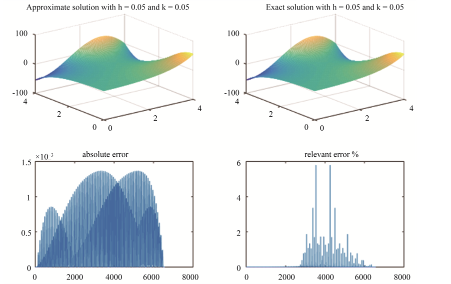
Figure 3. SCDM graphs.
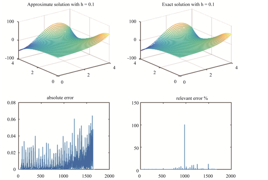
Figure 4. FEM graphs.
Approximate solution with h = 0.05 Exact solution with h = 0.05
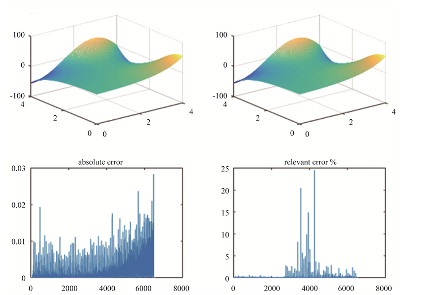
Figure 5. FEM graphs.
In Figure 6 and Figure 7 we have the graphs for SCDM and in Figure 8 and Figure 9 for FEM.
Example 3
Find the approximate solution of the partial differential equation

with Dirichlet boundary conditions along the rectangular domain

and exact solution

Table 4. Numerical results.
Table 5. Numerical results.
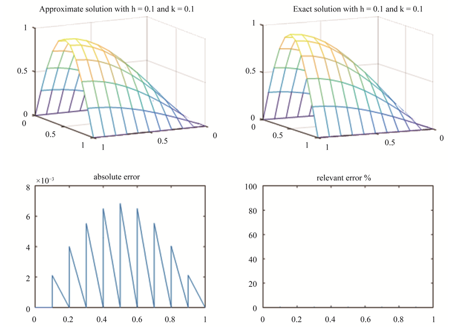
Figure 6. SCDM graphs.

Figure 7. SCDM graphs.
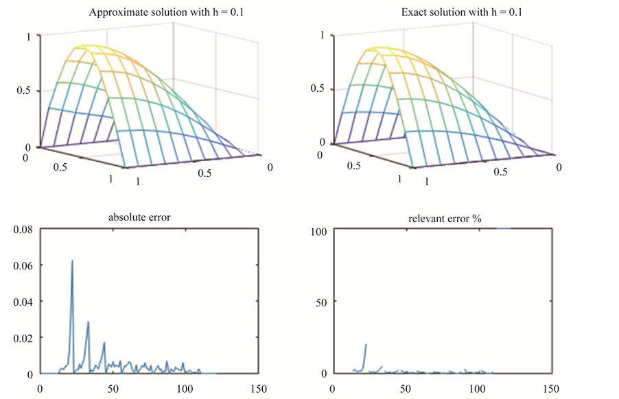
Figure 8. FEM graphs.
Approximate solution with h = 0.05 Exact solution with h = 0.05
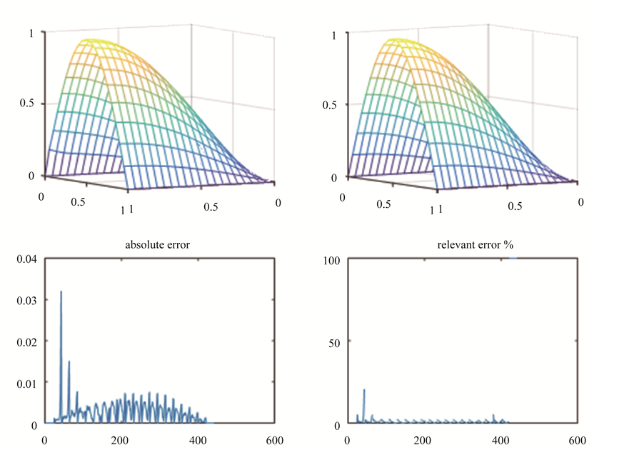
Figure 9. FEM graphs.
In Figure 10 and Figure 11 we have the graphs for SCDM and in Figure 12 and Figure 13 for FEM.
Overall, what stands out from these examples is that the finite element method has better approximations for the first problem compared to finite difference method for all the step-sizes that we have. But in the second problem we have a small difference in the results with better accuracy for the finite difference method and in the third problem the finite element method has bigger relevant errors than the difference method. More specifically, in example 1 according to the tables we have better approximations for the finite element method in both of step sizes and the mesh size parameters to specific points but the graphs of the percentage of relevant errors suggest that the second order central finite difference scheme produce better approximations generally. On the other hand, in the other two examples according to the tables and the graphs of errors in the second problem we have a small difference between these methods and in the third problem we have better approximations of the second order central difference scheme almost in all points of the domain. Conclusively, we can notice that in the third example for both of these methods the results which we obtained are almost identical when different step sizes are applied in CFDM and mesh size parameters in FEM.
Table 6. Numerical results.
Table 7. Numerical results.
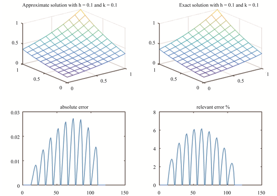
Figure 10. SCDM graphs.
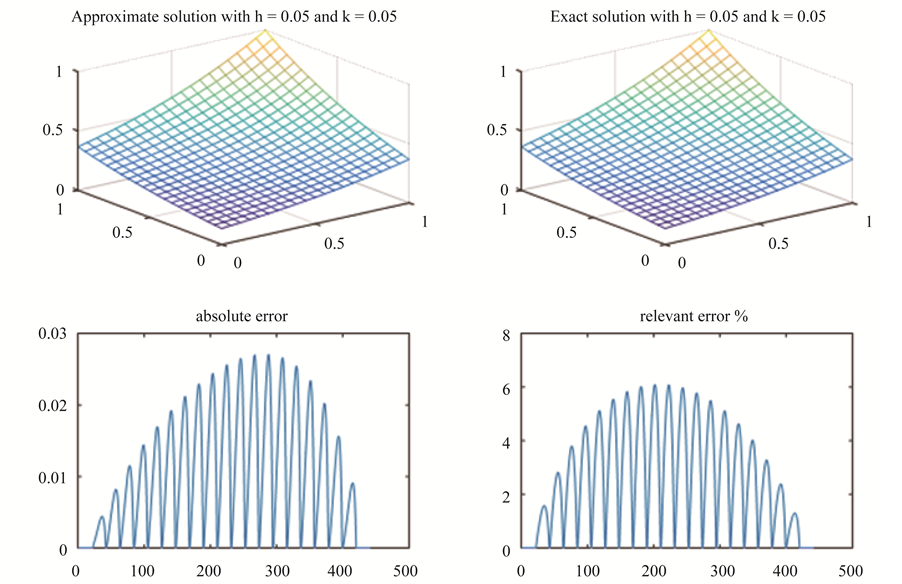
Figure 11. SCDM graphs.
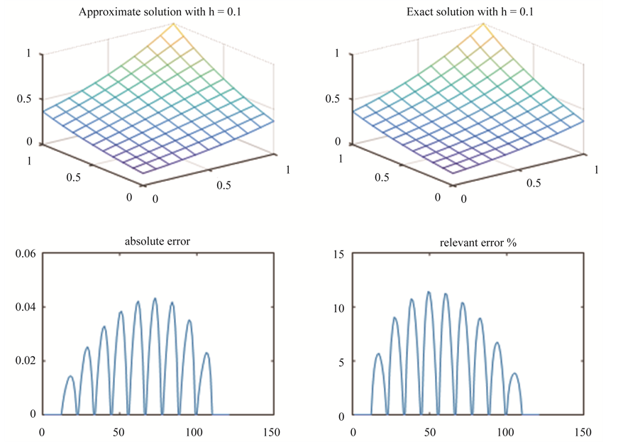
Figure 12. FEM graphs.
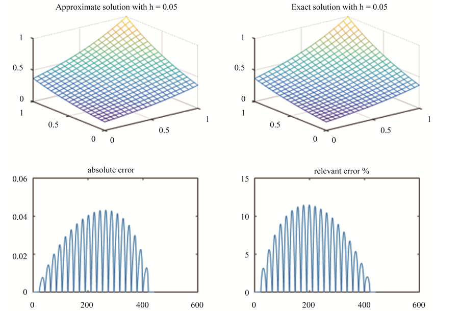
Figure 13. FEM graphs.
5. Conclusion
Finally, we can say that the data which we obtained from these examples show that both of these methods produce quite sufficient approximations for our problems. Also the results prove that the accuracy of them depends on the kind of the elliptical problem and the type of boundary conditions. For further research, the approximations of these methods can be improved. This improvement can be made if in the second order difference scheme we keep more taylor series terms in order to approximate the derivatives and in finite element method if we use higher order elements such as quadratic Lagrange triangular elements or cubic Hermite triangular elements.
Cite this paper
GeorgePapanikos,Maria Ch.Gousidou-Koutita, (2015) A Computational Study with Finite Element Method and Finite Difference Method for 2D Elliptic Partial Differential Equations. Applied Mathematics,06,2104-2124. doi: 10.4236/am.2015.612185
References
- 1. McDonough, J.M. (2008) Lectures on Computational Numerical Analysis of Partial Differential Equations.
http://www.engr.uky.edu/~acfd/me690-lctr-nts.pdf - 2. Gousidou-Koutita, M.C. (2014) Computational Mathematics. Tziolas, Ed.
- 3. Gousidou-Koutita, M.C. (2009) Numerical Methods with Applications to Ordinary and Partial Differential Equations. Notes, Department of Mathematics, Aristotle University of Thessaloniki, Thessaloniki.
- 4. Gousidou-Koutita, M.C. (2004) Numerical Analysis. Christodoulidis, K., Ed.
- 5. Dunavant, D.A. (1985) High Degree Efficient Symmetrical Gaussian Quadrature Rules for the Triangle. International Journal for Numerical Methods in Engineering, 21, 1129-1148.
http://dx.doi.org/10.1002/nme.1620210612 - 6. Reynolds, A.C., Burden, R.L. and Faires, J.D. (1981) Numerical Analysis. Second Edition. Youngstown State University, Youngstown.
- 7. Dougalis, V.A. (2013) Finite Element Method for the Numerical Solution of Partial Differential Equations. Revised Edition, Department of Mathematics, University of Athens, Zografou and Institute of Applied Mathematics and Computational Mathematics, FORTH, Heraklion.
- 8. Suli, E. (2012) Lecture Notes on Finite Element Method for Partial Differential Equations. Mathematical Institute, University of Oxford, Oxford.
- 9. Everstine, G.C. (2010) Numerical Solution of Partial Differential Equations. George Washington University, Washington DC.
- 10. Szabó, B. and Babuska, I. (1991) Finite Element Analysis. Wiley, New York.
- 11. Isaacson, E. and Keller, H.B. (1996) Analysis of Numerical Methods. John Wiley and Sons, New York.
- 12. Papanikos, G. (2015) Numerical Study with Methods of Characteristic Curves and Finite Element for Solving Partial Differential Equations with Matlab. Master’s Thesis.
- 13. Yang, W.Y., Cao, W., Chung, T.S. and Morri, J. (2005) Applied Numerical Methods Using MATLAB. John Wiley & Sons, Hoboken.
- 14. Gropp, W.D. and Keyest, D.E. (1989) Domain Decomposition with Local Refinement. Research Report YALEU/DCS/ RR-726.