Applied Mathematics
Vol.5 No.4(2014), Article ID:43580,16 pages DOI:10.4236/am.2014.54067
A Consecutive Quasilinearization Method for the Optimal Boundary Control of Semilinear Parabolic Equations
Mohammad Dehghan Nayyeri*, Ali Vahidian Kamyad
Applied Mathematics Department, Ferdowsi University of Mashhad, Mashhad, Iran
Email: *mu_de324@stu-mail.um.ac.ir, mudenayyeri@gmail.com, kamyad@math.um.ac.ir
Copyright © 2014 by authors and Scientific Research Publishing Inc.
This work is licensed under the Creative Commons Attribution International License (CC BY).
http://creativecommons.org/licenses/by/4.0/


Received 15 December 2013; revised 15 January 2014; accepted 23 January 2014
ABSTRACT
Optimal boundary control of semilinear parabolic equations requires efficient solution methods in applications. Solution methods bypass the nonlinearity in different approaches. One approach can be quasilinearization (QL) but its applicability is locally in time. Nonetheless, consecutive applications of it can form a new method which is applicable globally in time. Dividing the control problem equivalently into many finite consecutive control subproblems they can be solved consecutively by a QL method. The proposed QL method for each subproblem constructs an infinite sequence of linear-quadratic optimal boundary control problems. These problems have solutions which converge to any optimal solutions of the subproblem. This implies the uniqueness of optimal solution to the subproblem. By merging solutions to the subproblems, the solution of original control problem is obtained and its uniqueness is concluded. This uniqueness result is new. The proposed consecutive quasilinearization method is numerically stable with convergence order at least linear. Its consecutive feature prevents large scale computations and increases machine applicability. Its applicability for globalization of locally convergent methods makes it attractive for designing fast hybrid solution methods with global convergence.
Keywords:Quasilinearization; Optimal Boundary Control; SQP Methods; Semilinear Parabolic PDE’s

1. Introduction
The solution methods for the optimal control of nonlinear systems pass from nonlinearity to linearity in different approaches. For example the gradient methods modify iteratively the previous approximate solution by linearly seeking a suitable direction thorough solving a linear problem [1] . The SQP methods seek the optimal solution by linearizing the optimality systems using some version of Newton’s method [1] [2] . Our approach in this respect is to linearize the state equation through a quasilinearization method.
Quasilinearization method for nonlinear equations has its origin in the theory of dynamic programming and has important features in common with Newton’s method especially its form [3] . For a formal explanation let Y and Z be ordered Banach spaces,  be a bounded linear operator and
  be a nonlinear differentiable operator. Consider the equation
 (1.1)
(1.1)
In the convex case , Equation (1.1) can be written as
 (1.2)
(1.2)
where the right hand side is quasilinear. Then starting from  thorough the quasilinearization method, a sequence of linear equations is defined
 (1.3)
(1.3)
which produces the sequence of approximate solutions  in
in , converging to
 , the solution of (1.2) or (1.1); see [3] [4] . This method has the following features. 1)
  is monotonic. This stems from positivity and inverse positivity of
  and
and . 2) the convergence is globally in the sense that
  can be any lower solution of (1.1), i.e.
 . 3) The rate of convergence is quadratic. For details on these features refer to [3] [5] . There are some extensions, refinements and generalizations to the quasilinearization method which preserve the above features but relax the convexity assumption on
 ; for a complete survey see [5] -[7] . Quasilinearization method has intimate connection with the theory of positive and monotone operators, maximum operation and differential inequalities; confer [8] , Sec. 4.33; [4] [9] .
In order to introduce the proposed consecutive quasilinearization method for optimal control problems let  be a Banach space,
  be a functional and
  be a bounded linear boundary operator. Consider the following optimal boundary control problem:
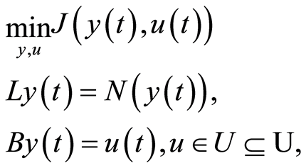 (1.4)
(1.4)
where  belongs to a time interval
 . For
. For  consider the following approximation to (1.4):
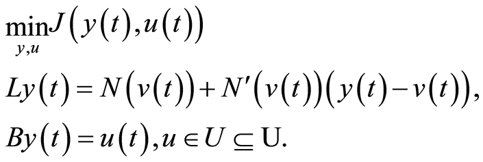 (1.5)
(1.5)
Starting from , let
, let  be the optimal solution of (1.5) with
 . Then the sequence
  converges to the solution of (1.4) with the following features: 1) The convergence is occurred for
 , for some
 . 2) The convergence is globally in the sense that
  can be chosen any element in a subspace of
 . 3) The rate of convergence is at least linear but it is not necessarily super-linear or quadratic. Here the sequence
  or
or  is not necessarily monotonic even when
  is convex or concave. For the case
  the optimal control problem is decomposed into many finite optimal control subproblems each on a time interval with length less than some
  and then the above method be applied to each of them consecutively. Here
  is such that the stability is preserved.
The optimal boundary control problem which is investigated has the standard quadratic objective of tracking type and a state constraint comprised of a semilinear parabolic equation with mixed boundary type. For such control problems, due to lack of convexity of the solution set, there is no general uniqueness result based on the optimality theory of optimal control problems [1] [2] [10] . However, a uniqueness result for such problems is obtained here as a by-product of the convergence of proposed consecutive quasilinearization method.
The organization of paper is as follows. Section 2 introduces the state equation and some estimates concerning solution of linear initial-boundary value problems. Section 3 proves the existence of an optimal solution. Section 4 introduces the quasilinearization method and proves its convergence for . Section 5 explains how to apply the quasilinearization method consecutively to the optimal boundary control problem when
 . Also the uniqueness of optimal solution is stated there. In Section 6 the error and stability analysis of consecutive quasilinearization method is investigated. Section 7 presents a numerical example concerning the obtained results.
2. The State Equation
Let  be an open bounded domain in
 ,
,  , with boundary
  of class
  for some
 . Let
. Let ,
,  and
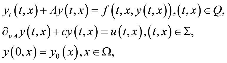
and . Consider the control system described by the semilinear parabolic initial-boundary value problem:
 (1.6)
(1.6)
where  and
and  are, respectively, the state and the distributed control of system,
  is the system nonlinearity and
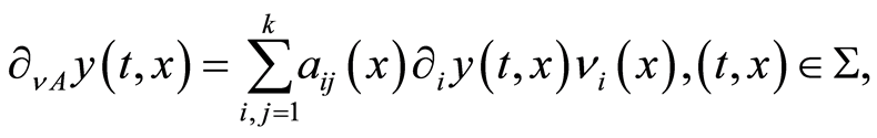
is the normal derivative of  associated with
  wherein
  is the outward unit normal to
 .
.
The following assumptions are imposed on the system and data:
• (A1)  is a secod order differential operator in divergence form:
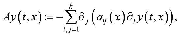 (1.7)
(1.7)
where  and
and  is uniformly elliptic, i.e. for every
 ,
,
 (1.8)
(1.8)
for some . Also it is considered
 .
.
• (A2)  satisfies Caratheodory’s condition, i.e.
  is measurable on
  and continuous on
 , and the Nemytskii’s operator
 , defined by
  , is bounded and continuous. A sufficient condition for that is
 (1.9)
(1.9)
for some , Theorem 3.2 in [11] .
• (A3)  is twice continously differentiable with respect to
  and
and
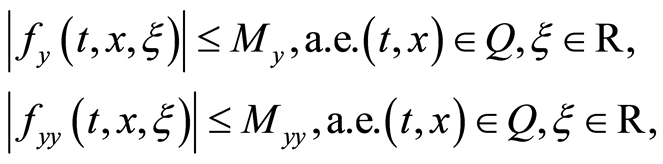
for constants ,
, .
.
The standard function spaces ,
,  and
and  are used in the paper. Identifying
  with its dual
  results in the evolution triples
  , where the embeddings are dense, continuous and compact. The standard solution space of parabolic problems and its norm is defined as
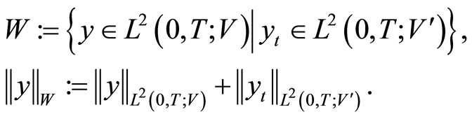
The continuous embeddings  and
and  are well-known and the latter is compact. For detailed definitions and properties of the above spaces refer to [11] -[14] .
The bilinear form associated with Equation (1.6) is defined as follows:
 (1.10)
By Assumption (A1) the coefficients in (0.10) are bounded. This results in the boundedness of . Let
. Let  denotes the duality pairing between
  and its dual
 , and
, and  and
and  denote respectively the inner product of
  and
and . Then Definition 1 Let
 . For
. For  a function
  is called a weak solution of (0.6) if
  and
and
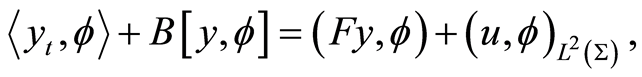
for all .
.
Next theorem under weaker assumptions is proved in Theorem 3.1 of [10] .
Theorem 1 Let . Then under Assumptions (A1)-(A3) for every
  problem (0.6) admits a unique weak solution
 .
.
In the following sections the linear initial-boundary value problems of the type below are used:
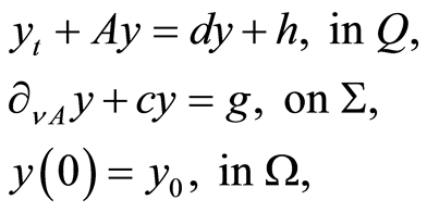 (1.11)
where ,
,  ,
,  ,
,  and
and . Define the family of bilinear forms
 , a.e.
 , by
, by
 (1.12)
By Assumption (A1) the coefficients in (0.12) are bounded for a.e. . Thus
  is bounded on
  for a.e.
 . Let
. Let  be the duality pairing between
  and its dual
 , and
, and  and
and  be the inner product of
  and
and .
.
Definition 2 A function  is called a weak solution of (0.11) if
  and
and

for all  and a.e.
 .
.
Norm estimates concerning solution of problem (1.11) are common in the literature of linear initial-boundary value problems [12] -[14] . Next theorem states some of them clarifying the time dependency quality of their constants. Its proof has been included due to lack of suitable reference, on the best of our knowledge, for the form stated here.
Theorem 2 The initial-boundary value problem (0.11) has a unique weak solution  with norm estimates
 (1.13)
 (1.14)
 (1.15)
where  and
and  are bounded when
  varies boundedly and
 . If
. If ,
,  and
and  then
then .
.
Proof 1 By Theorem 5.3 in Ch. III of [15] for some  the following estimate exists:

Using the Garding inequality (Proposition 22.45 in [14] ) or the elliptic energy estimates (Sec. 6.2.2, Theorem 2 in [12] ) it is obtained
 (1.16)
for a.e. , where
  and
and . Then the existence of a unique weak solution
  of (1.11) which satisfies the estimate (1.13) is deduced using a Galerkin procedure (Proposition 23.30 in [14] ).
To obtain estimates (1.14) and (1.15) let  be the weak solution of (1.11). Then Definition 2 with
  yields
 (1.17)
Furthermore,
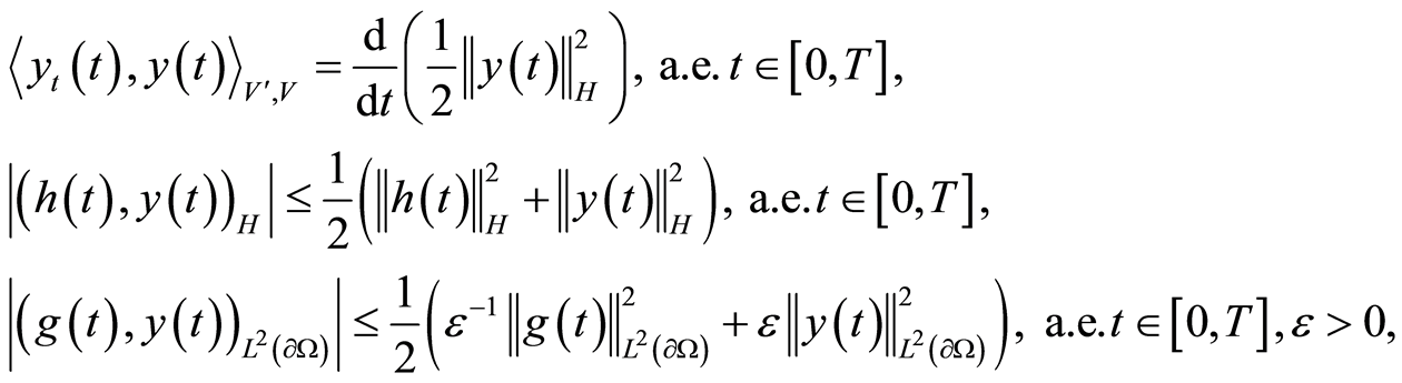 (1.18)
where the equation is proved in Ch. III, Proposition 2.1 [11] and the inequalities are obtained by Cauchy’s inequality. The continuous embedding  yields
 ,
,  , for some
 , Ch. II, Theorem 3.3 in [11] .
Consequently, (0.16)-(0.18) with  yield
yield
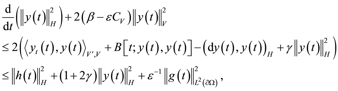 (1.19)
for a.e. . Now let
  and
and . Then (1.19) implies

and the differential form of Gronwall’s inequality (Appendix B2 [12] ) yields
Since  it is obtained
 (1.20)
Integrating (1.20) from  to
to , results
By employing the inequality , the estimate (1.14) with
  is concluded and
 .
.
The estimate (1.15) is a consequence of (1.20) with . The last assertion of Theorem is proved in Proposition 3.3 of [10] .
We also meet the backward form of problem (1.11), i.e. the linear final-boundary value problem,
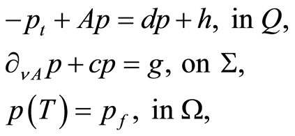 (1.21)
with ,
,  ,
,  ,
,  and
and . All results of Theorem 2 are valid for (0.21).
Theorem 3 The initial-boundary value problem (1.21) has a unique weak solution  with norm estimates
 (1.22)
 (1.23)
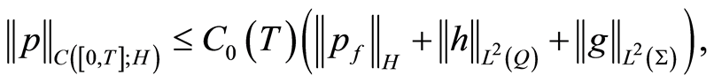 (1.24)
where  and
and  are bounded when
  varies boundedly and
  . If
. If ,
,  and
and  then
then .
.
Proof 2 The substitution  in (0.21) yields the following equivalent problem to the problem (0.11) in the forward form
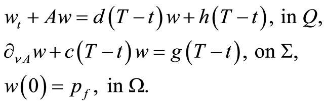 (1.25)
Problem (1.25) satisfies all the assumptions which problem (1.11) satisfies. Therefore the assertions of Theorem 2 and the estimates (1.13)-(1.15) are valid for . Since
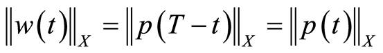 , when
  is one of spaces
 ,
,  ,
,  or
or , the assertions of theorem and the estimates (1.22)-(1.24) are verified.
3. The Optimality System
Let  with
with . Consider the following control problem
 (1.26)
where  and
and .
.
Theorem 4 Under Assumptions (A1)-(A3) the optimal control problem (0.26) has an optimal solution  in
in .
.
Proof 3 By Theorem 1 the optimal control problem (0.26) is feasible. Also the Nemytskii operator
 ,
,  , as an operator from
  into
into  is completely continuous. Because, when
 , weakly in
 , the compact embedding
  yields
 , strongly in
 . Consequently, the continuity of
  and the continuous embedding
  results in
  , strongly in
 , (confer Assumption (A2)).
Thus, the existence of an optimal solution  for the problem (1.26) can be deduced from Theorem 1.45 of [1] .
Theorem 5 A necessary condition for  be a local solution (or an optimal solution) of problem (0.26) is that there exists
  such that
 (1.27)
 (1.28)
 (1.29)
Proof 4 Corollary 1.3 in [1] (or Theorem 1.48 in [1] ).
Theorem 6 Any solution  of the optimality system (1.27)-(1.29) belongs to
 .
.
Proof 5 As  is bounded, utilizing Theorem 2.1 (or Theorem 3.1 in [10] ) it is deduced
 . Then Theorem 2.1 in [10] yields
 .
.
Lemma 1 The optimality condition (0.29) can be written in the equivalent form bellow:
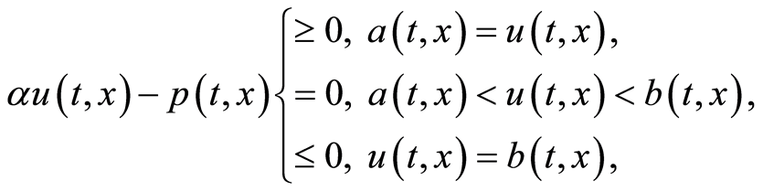 (1.30)
for a.e. .
.
Proof 6 Refer to Lemma 1.12 in [1] .
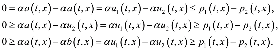
Corollary 1 Let ,
,  , satisfy (0.30). Then
 (1.31)
( ’s and
 ’s do not necessarily satisfy an optimality system).
Proof 7 Let  and
and ,
,  , satisfy (0.30) at
 . Then one of the three cases below occurs for
  at
at ,
,
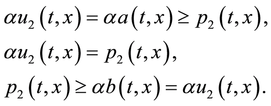
Similarly one of the three such cases occurs for  at
at . Let the first case be occurred for
  at
at . Then one of the three cases below must be considered for
  at
at ,
,
As you see each of the three cases above satisfies (0.31) at . In a similar argument for each of the two other cases of
  at
at , three relations as the above can be written proving that each of them satisfy (0.31) at
 .
.
4. The Quasilinearization Method
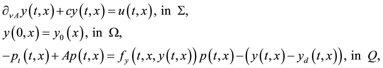
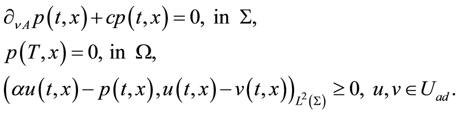
Consider problem (1.26) under Assumptions (A1)-(A3). We investigate instead of the optimality system (1.27)- (1.29) the following one wherein the optimality condition (1.29) has been replaced by its equivalent form (1.30), confer Lemma 1:
 (1.32)
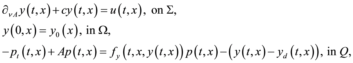 (1.33)
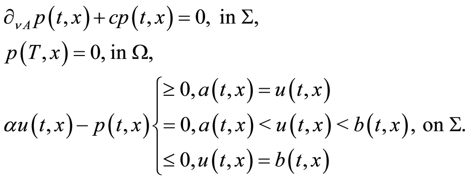 (1.34)
By Theorem 5 and Theorem 4 optimality system (1.32)-(1.34) has at least one solution.
Theorem 7 Let  be a solution of optimality system (0.32)-(0.34). Then there exists a sequence
  in
in  whose elements are the unique solution of the following linear optimality systems and there exists
  such that this sequence converges, at least linearly, to
  when
when . As a consequence when
  optimality system (1.32)-(1.34) has a unique solution.
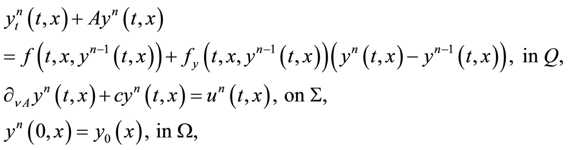 (1.35)
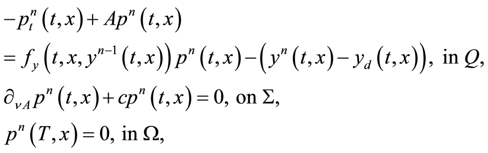 (1.36)
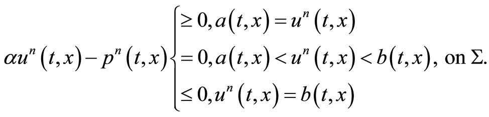 (1.37)
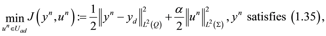
Proof 8 About the existence of sequence  in
in , note that (0.35)-(0.37) is the optimality system of following linear-quadratic optimal control problem
 (1.38)
which has a unique optimal solution (Theorem 1.43 [1] ). Then the optimality theory for linear-quadratic optimal control problems yields the existence of a unique solution  in
in  of the system (1.35)- (1.37) when
 , confer Sections 1.5-1.7 in [1] . Referring to Theorems 2 and 3 it is deduced
  and
and .
.
Now let  be a solutions of the optimality systems (1.32)-(1.34). Define
 (1.39)
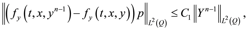
Then (1.32) and (1.35) and the mean value theorem yield
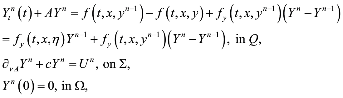 (1.40)
where  lies between
  and
and ,
, . By Assumption (A3),
 . Thus considering (1.40) as the linear problem (1.11) with
 , it is concluded by Theorem 2,
 (1.41)
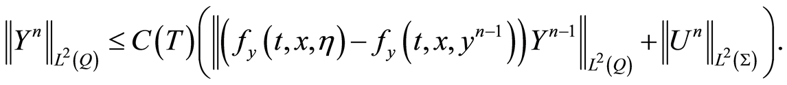
Also (1.33) and (1.36) yield
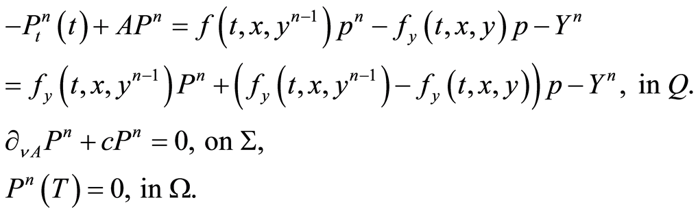 (1.42)
Since , considering (1.42) as the linear problem (1.21) with
 , it is concluded by Theorem 3,
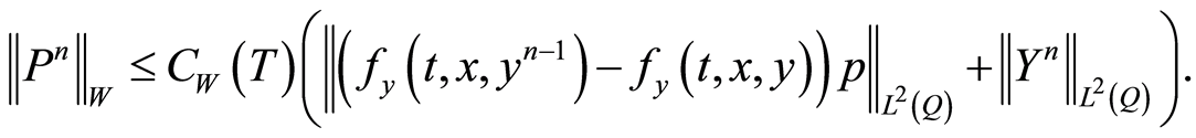 (1.43)
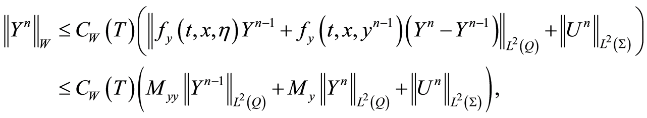
Referring to Theorem 4,  belongs to
 . Consequently employing Assumption (A3) and the mean value theorem, it is obtained
 (1.44)
where  in which
  lies between
  and
and ,
, . Therefore (1.43) yields
 (1.45)
Owing to Corollary 1 and the continuous embeddings 
 (1.46)
Now combining (1.41), (1.45) and (1.46) results in

Consequently, it is obtained
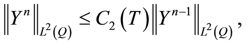 (1.47)
wherein
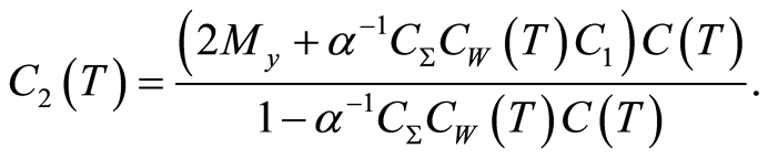 (1.48)
Referring to Theorem 2,  when
when  and
and  is bounded. Consequently, there exists
  such that for
  the denumerator in (1.48) be positive and
 . This yields the convergence of
  to zero in
  for
for , thereby the convergence of
  to zero in
  for
for  via (1.45) and the convergence of
  to zero in
  for
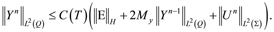
for  via (1.46). The estimate (1.13) in Theorem 2 for the initial boundary value problem (1.40) yields
 (1.49)
where the second inequality is obtained using the mean value theorem. Consequently, the convergence of  to zero in
  for
for  is obtained. Referring to (0.47), the convergence of
  in
in  is at least linear whereby the convergence of
  in
in  and
and  in
in  will be at least linear for
 , confer (1.45) and (1.46). Then it is concluded from the estimates (1.49) that the convergence rate of
  to zero in
  is at least linear for
 .
.
The sequence  produced by (1.35)-(1.37) is independent from
  and converges to it in
 . As
. As  can be any solution of optimality system (1.32)-(1.34) this is impossible except optimality system (1.32)-(1.34) has only one solution.
The next two corollaries are used in the error analysis in Section 6.
Corollary 2 Under assumptions of Theorem 7 there exists ,
,  , such that for
  the following estimate is valid
 (1.50)
where ,
,  and
and  are as in (1.39), (1.48) and (1.53), respectively.
Proof 9 The proof follows the lines of proof of Theorem 7. As  satisfies (0.40) the estimate (0.15) in Theorem 2 yields
 (1.51)
Next employing the estimates (1.45) and (1.46) result in

As  it is deduced from the above inequality
 (1.52)
wherein
 (1.53)
Referring to Theorem 2,  and
and  are bounded when
  whereby there exists
  such that the denumerator in (1.53) is positive for
 . Set
. Set  with
with  being determined in Theorem 7. Then (1.50) is obtained from (1.52) by repeatedly employing the estimate (1.47).
Corollary 3 Suppose in the quasilinearization method in Theorem 7 instead of the accurate initial value  the approximate initial value
  is used. Let
  be as in Corollary 2. Then for
  the following estimate is valid
 (1.54)
where ,
,  and
and  are as in (1.48), (1.53) and (1.59), respectively.
Proof 10 The proof follows the lines of proof of Theorem 7. As  satisfies (1.40) in
  with
with  the estimate (1.15) in Theorem 2 yields
 (1.55)
Next employing the estimate (1.45) and (1.46) result in

As , choosing
  as in Corollary 2, (0.55) for
  yields
 (1.56)
where .
.
Now in order to conclude (0.54) we need an estimate like (1.47). (1.47) is for the case  here
here . Such an estimate is obtained following the lines which (1.47) obtained. As
  satisfies (1.40) with
 , the estimate (1.14) in Theorem 2 yields
Then employing the estimates (1.45) and (1.46) result in

where ,
,  being determined after (1.48). Referring to (1.48), without loss of generality, it is considered
 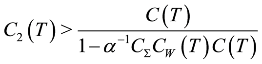 whereby it is obtained
 (1.57)
Employing repeatedly (0.57) yields
 (1.58)
where the last inequality is obtained from  for
for . Now utilizing (1.58) in (1.56) results in (1.54) with
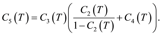 (1.59)
5. Application to the Optimal Boundary Control Problems and the Uniqueness
The proposed quasilinearization method in Theorem 7 is convergent on the time intervals  for
for ,
,  being determined in Theorem 7. In order to apply the quasilinearization method to the optimal control problem (1.26) up to an arbitrary final time
  it is possible to decompose the problem into many finite optimal control problems each on an interval with length less than
 . In order to follow such an approach let
  1
1
and  for some
 . Let
. Let ,
,  and
and ,
, . Let
. Let  be a Banach space. Then
  is normisomorphic to
  through the isomorphism
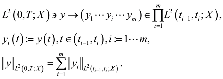
Replacing  by
by  yields that
  be normisomorphic to
  with the norm identity
 , and replacing
  by
by  yields that
  be normisomorphic to the closed subspace
  of
of  with the norm identity
 , where

Thus, if  satisfies the initial-boundary value problem (0.6) then
 ,
,  , satisfy consecutively the following initial-boundary value problems and vice versa:
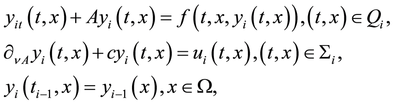 (1.60)
wherein . Consequently, the optimal control problem (1.26) is equivalent to the consecutive optimal control subproblems
 (1.61)
wherein . Therefore, solving the optimal control problem (1.26) is equivalent to consecutively solving the optimal control subproblems (1.61). Furthermore, the proposed quasilinearization method in Theorem 7 is applicable to each optimal control subproblem in (1.61). In fact the substitution
  in the
  -th subproblem in (1.61) transforms it into an equivalent problem on the time interval
  whereby the quasilinearization method will be applicable to it.
Moreover, as a consequence of Theorem 7 the solution of optimality system of  -th subproblem in (1.61) is unique. Thus, in view of Theorem’s 4 and 5, each subproblem in (1.61) has a unique optimal solution. Consequently by the equivalence between problem (1.26) and consecutive subproblems (1.61) it can be stated Theorem 8 Optimal boundary control problem (1.26) under Assumptions (A1)-(A3) has unique optimal boundary control solution and optimal state solution.
Note that the uniqueness could not be established thorough the optimality theory of optimal control problems which was used for stating the existence in Section 3. This is due to lack of convexity of the solution set of problem (1.26).
An issue concerning the above consecutive process is the relation between , the solution of optimality system of problem (1.26), and
 , the solution of optimality system of
  -th subproblem in (1.61).
  satisfies (1.27)-(1.29) on
  and
and  satisfies
 (1.62)
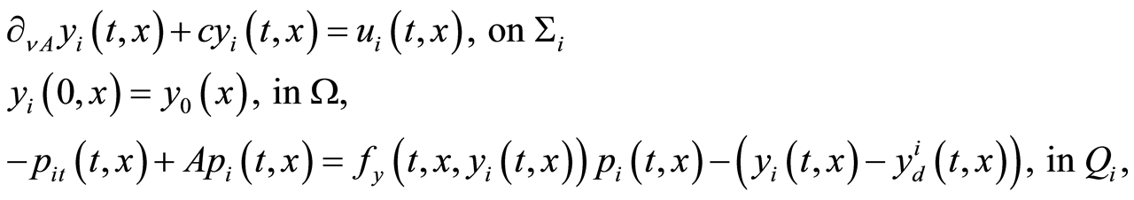 (1.63)
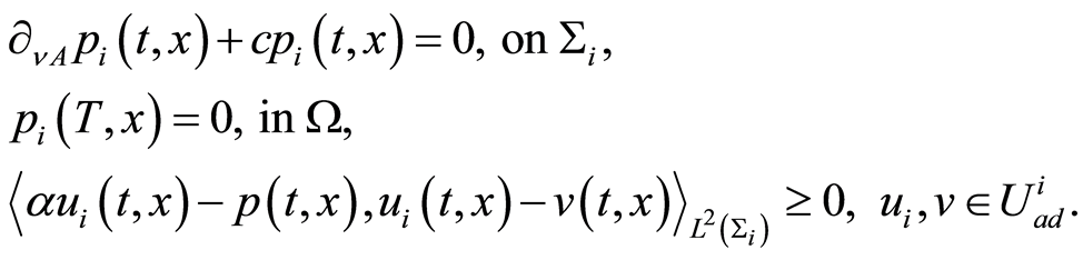 (1.64)
In view of Theorem’s 8, 4 and 5 optimality system of problem (1.26) has a unique solution. Consequenty comparing (1.61)-(1.64) with (1.26)-(1.29) it is concluded that 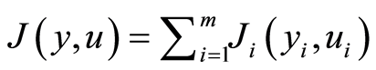 and
and ,
,  , and
, and ,
, . But there is not a similar relation between the costates
  and
and
 ’s, since
  satisfies (1.63) and
 , but
, but  is not necessarily zero; confer (1.28). Also it is not possible in general to construct
  from
from ’s; however, after obtaining
 ’s,
’s,  can be computed from (1.28).
6. Error Analysis
By the consecutive quasilinearization method in Section 5, the optimal control problem (1.26) is solved through m consecutive optimal control subproblems (1.61). Each subproblem is solved by the quasilinearization method in Theorem 7 which is an iterative method with infinite iterations. In applications it is implemented up to a finite iterations, thereby producing error. Consequently, during solving each subproblem there exists an error production and an error propagation.
Let  be the solution of optimality system (1.32)-(1.34),
  be the solution of i-th optimality system (0.62)-(0.64) and
  be the solution provided by the quasilinearization method at iteration n for the i-th optimality system, i.e. one which satisfies (1.35)-(1.37) on
 . For the first subproblem the quasilinearization method starts with the accurate initial value
  and it is terminated after N iteration with the final value
 . The error equals to
 . As
. As  and the initial value is accurate, Corollary 2 with
  yields
 (1.65)
For the i-th subproblem on ,
,  , the quasilinearization method starts with the approximate initial value
  and it is terminated after N iteration with final value
 . The error of final value equals to
 . Next, we estimate this error.
The substitution  in the i-th subproblem in (1.61) transforms it into an equivalent problem on the time interval
 . Setting
  and utilizing Corollary 3 for the equivalent problem, yields the estimate (1.54) with
 . Then utilizing the reverse substitution
  results in the estimate
 (1.66)
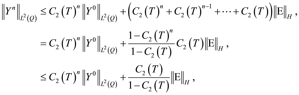
Now beginning from  down to
 , repeatedly employing (1.66) results in
where the last inequality is obtained by  and the estimate (1.65). Consequently,
 (1.67)
Note that  presents the accumulated error consists of the production errors and the propagation errors in the consecutive implementation of m quasilinearization method, when the implementation is up to N iteration on each subproblem. In the estimate (1.67) the term
  is independent from N and
 ; confer (1.48) and thereafter. Since m is fixed, by increasing the number of iterations N, the total accumulated error
  tends to zero in H. Therefore, the proposed consecutive quasilinearization method in Section 5 is stable. Furthermore,
  for
for , although
  and
and  decrease when T decrease (or m increase). Consequently it may a trade off be necessary between size of m (the number of subproblems) and N (the number of required iterations in the implementation of quasilinearization method) in order to have the desired total error in the consecutive quasilinearization method.
7. Numerical Example
A typical example is presented reflecting the obtained results in the previous sections in applications. Consider the optimal control problem (1.26) with the following data: ,
,  ,
,  ,
,
 ,
,  ,
,  ,
,  ,
,  ,
,  ,
,
 ,
, . Setting
 , the consecutive quasilinearization method is implemented on the m consecutive subproblems (1.61) with the optimality systems (1.62)-(1.64). The corresponding states
 , costates
  and controls
  are approximated by the elements and boundary elements of continuous linear finite element spaces on
  with
with  and
and , i.e. without discretization of time. The linear optimality systems (1.62)-(1.64) are solved by the semismooth Newton’s method [16] or Section 2.5 in [1] , and the implementation is done with MATLAB software. Table 1 presents the values of
 ,
,

and
 .
.
These values present at least a linear rate of convergence in the quasilinearization method as it was deduced from (1.45)-(1.47).
Table 2 presents the optimal objective values of problem when the consecutive quasilinearization method is implemented with different number of subproblems but fixed number of iterations in each quasilinearization

Table 1. The difference between iterations in the quasilineariztion method for the forth subproblem at t = t4 when m = 15 and the number of iterations is N = 10.
Table 2. The optimal objective values with different number of subproblems, m, but fixed number of iterations in the quasilinearization method, i.e. N = 5.
method, i.e. with different m’s and fixed N. As  is in some sense the step size of time discretization, its increment yields more accurate approximation to the optimal objective value.
8. Conclusions
A consecutive quasilinearization method was proposed for the optimal boundary control problems with quadratic objective of tracking type and a semilinear parabolic equation with mixed boundary as the state constraint; cf.
(1.26) and (1.32). The proposed method divides the control problem equivalently into many finite consecutive subproblems through partitioning the time interval into subintervals; cf. Section 5 and (1.61). Then subproblems are solved consecutively by a quasilinearization method (hence the name of proposed method). Finally the optimal solution of control problem is obtained by consecutively merging optimal solutions of subproblems. The quasilinearization method for each subproblem constructs an infinite sequence of linear-quadratic optimal boundary control problems of form (1.38). The sequence of solutions to the optimality systems of these linear problems converges to any solutions of the optimality system of subproblem; confer Theorem 7 and Section 5. This implies the uniqueness of solution to the optimality system of a subproblem, hence the uniqueness of optimal solution to the original control problem; confer Theorem 8. This uniqueness result is new, on the best of our knowledge, in the class of optimal control problems with state constraint of semilinear parabolic equation type.
The convergence of quasilinearization method for each subproblem depends on the time interval length of the subproblem,  , and there is a bound on
  which the convergence occurs,
  ,
,  being determined in Theorem 7. In comparison with methods which require the fully discretization of original control problem, cf. Chapter 2 in [1] , [2] and [17] ,
  can be considered as the time discretization step length. In this view the consecutive feature of proposed method replaces the large scale computations in fully discrete methods by the consecutive small scale computations in the subproblems, hence increasing the machine applicability of method. Specially in quasilinearization method in solving the sequence of linear-quadratic control problems the time discretization can be avoided by choosing
  enough small , cf. Section 7.
In comparison with superlinear methods which are locally convergent, as different versions of Newton’s method and/or Lagrange-SQP methods (Chapter 2 in [1] , and [2] ), the consecutive quasilinearization method is globally convergent and its convergence order is at least linear, cf. Theorem 7. For example Table 1 of Section 7 presents a cubic convergence rate. Thereby the consecutive quasilinearization method is very suitable for the globalization of locally convergent methods by applying it to find a starting solution for those methods.
The quasilinearization method for subproblems has infinite iterations, but in applications it is implemented up to a finite iteration. Therefore its consecutive application on the subproblems produces and propagates errors. However choosing  guarantees the numerical stability, cf. Section 6.
The imposed boundedness assumptions on the nonlinearity of problem and the admissible controls are necessary for the convergence proof, cf. Assumption (A3), Section 3 and proof of Theorem 7. As the investigated control problem here also has optimal solution with much weaker boundedness assumptions, cf. [10] , application of consecutive quasilinearization method in this case requires new convergence proof.
References
- Hinze, M., Pinnau, R., Ulbrich, M. and Ulbrich, S. (2009) Optimization with PDE Constraints. Springer, Berlin.
- Trötzsch, F. (1999) On the Lagrange-Newton-SQP Method for the Optimal Control of Semilinear Parabolic Equations. SIAM Journal on Control and Optimization, 38, 294-312. http://dx.doi.org/10.1137/S0363012998341423
- Bellman, R. and Kalaba, R. (1965) Quasilinearization and Nonlinear Boundary-Value Problems. American Elsevier Publishing Company, New York.
- Bellman, R. (1955) Functional Equations in the Theory of Dynamic Programming. V. Positivity and Quasi-Linearity. Proceedings of the National Academy of Sciences of the United States of America, 41, 743-746. http://dx.doi.org/10.1073/pnas.41.10.743
- Buica, A. and Precup, R. (2002) Abstract Generalized Quasilinearization Method for Coincidences. Nonlinear Studies, 9, 371-386.
- Lakshmikantham, V. and Vatsala, A.S. (1995) Generalized Quasilinearization for Nonlinear Problems. Kluwer Academic Publishers, Dordrecht.
- Carl, S. and Lakshmikantham, V. (2002) Generalized Quasilinearization and Semilinear Parabolic Problems. Nonlinear Analysis, 48, 947-960. http://dx.doi.org/10.1016/S0362-546X(00)00225-X
- Beckenbach, E.F. and Bellman, R. (1961) Inequalities. Springer-Verlag, Berlin.
- Kalaba, R. (1959) On Nonlinear Differential Equations, the Maximum Operation, and Monotone Convergence. Journal of Mathematics and Mechanics, 8, 519-574.
- Raymond, J.P. and Zidani, H. (1999) Hamiltonian Pontryagin’s Principles for Control Problems Governed by Semilinear Parabolic Equations. Applied Mathematics and Optimization, 39, 143-177. http://dx.doi.org/10.1007/s002459900102
- Showalter, R.E. (1997) Monotone Operators in Banach Spaces and Nonlinear Partial Differential Equations. American Mathematical Society, Providence.
- Evans, L.C. (1998) Partial Differential Equations. American Mathematical Society, Providence.
- Ladyzenskaja, O.A., Solonnikov, V.A. and Ural’ceva, N.N. (1968) Linear and Quasi-Linear Equations of Parabolic Type. American Mathematical Society, Providence.
- Zeidler, E. (1990) Nonlinear Functional Analysis and Its Applications Vol II/A: Linear Monotone Operators. Springer, Berlin.
- Showalter, R.E. (1994) Hilbert Space Methods for Partial Differential Equations. Electronic Journal of Differential Equations, Monograph 01, Dover Publications, Mineola.
- Ulbrich, M. (2011) Semismooth Newton Methods for Variational Inequalities and Constrained Optimization Problems in Function Spaces. SIAM. http://dx.doi.org/10.1137/1.9781611970692
NOTES
*Corresponding author.
1In order to preserve the stability, T2 is chosen as in Corollary 2 (also confer Section 6).