Applied Mathematics
Vol.3 No.9(2012), Article ID:23011,15 pages DOI:10.4236/am.2012.39154
Analytical Solutions of Some Two-Point Non-Linear Elliptic Boundary Value Problems
Department of Mathematics, The Madura College, Madurai, India
Email: *raj_sms@rediffmail.com
Received July 16, 2012; revised August 16, 2012; accepted August 23, 2012
Keywords: Two-Point Elliptic Boundary Value Problems; Bratu’s Equation; Troesch’s Problem; Non-Linear Equations; Homotopy Perturbation Method; Porous Catalyst; Numerical Simulation
ABSTRACT
Several problems arising in science and engineering are modeled by differential equations that involve conditions that are specified at more than one point. The non-linear two-point boundary value problem (TPBVP) (Bratu’s equation, Troesch’s problems) occurs engineering and science, including the modeling of chemical reactions diffusion processes and heat transfer. An analytical expression pertaining to the concentration of substrate is obtained using Homotopy perturbation method for all values of parameters. These approximate analytical results were found to be in good agreement with the simulation results.
1. Introduction
All chemical reactions are usually accompanied with mass and energy transfer, either homogeneously or heterogeneously. Mathematical modeling for these processes is based on material and energy balance. One can generate a set of differential equations known as the reaction-diffusion problem. Owing to the strong nonlinearity of the reaction rate, mainly from the effect of temperature, reaction-diffusion equations are paid more attention in analyzing and designing chemical and catalytic reactors [1]. The same phenomena exist in electrochemical processes, with the add complexity of a varying potential field, and considerable research has been reviewed for electrochemical reactions occurring in the porous electrode [2].
Linear and nonlinear phenomena are of fundamental importance in various fields of science and engineering. Most models of real-life problems are still very difficult to solve. Therefore, approximate analytical solutions such as Homotopy perturbation method (HPM) [3-12] were introduced. This method is the most effective and convenient ones for both linear and nonlinear equations. Perturbation method is based on assuming a small parameter. The majority of nonlinear problems, especially those having strong nonlinearity, have no small parameters at all and the approximate solutions obtained by the perturbation methods, in most cases, are valid only for small values of the small parameter. Generally, the perturbation solutions are uniformly valid as long as a scientific system parameter is small. However, we cannot rely fully on the approximations, because there is no criterion on which the small parameter should exists. Thus, it is essential to check the validity of the approximations numerically and/or experimentally. To overcome these difficulties, HPM have been proposed recently. In this paper we will apply Homotopy perturbation method (HPM) to the nonlinear Bratu’s problem, Troesch’s problem, and catalytic reactions in flat particles.
Systems of non linear differential equations arise in mathematical models throughout science and engineering. When an explicit condition that a solution must satisfy is specified at one value of the independent variable, usually its lower bound, this is referred to as an initial value problem (IVP). When the conditions to be satisfied occur at more than one value of the independent variable, this is referred to as a boundary value problem (BVP). If there are two values of the independent variable at which conditions are specified, then this is a two-point boundary value problem (TPBVP). TPBVPs occur in a wide variety of problems, including the modelling of chemical reactions, heat transfer, and diffusion. They are also of interest in optimal control problems.
There are many techniques available for the numerical solution of TPBVPs for ordinary differential equations [13]. The standard techniques can be divided into two classes. Typical of this class are various shooting and multi-shooting approaches. The other class involves converting the TPBVP into a system of algebraic equations, and includes methods based on various versions of finite difference or collocation. Methods for solving TPBVPs usually require users to provide an initial guess for the unknown initial states and/or parameters.
The problem of reliably identifying all solutions of a TPBVP was apparently first addressed only recently, by [14,15]. Present a new approach that will rigorously guarantee the enclosure of all solutions to the TPBVP. In this paper we have obtained the analytical solutions of some nonlinear elliptic problems (Bratu’s equation, Troesch’s problem and Catalytic reactions in a flat particles) using Homotopy perturbation method.
2. Mathematical Formulation of the Problem
Many problems in science and engineering require the computational of family of solutions of a non linear system of the form [16]:
 (1)
(1)
where  is continuously differentiable function, y represents the solution and
  is a real parameter (i.e., Reynold’s number, load etc.). It is required to find a solution for some
  -interval, i.e., a path solutions,
 . Equations of the form (1) are called nonlinear elliptic eigenvalue problems if the operator G with
  fixed is an elliptic differential operator. Fore more details about this type of operators see [17]. As a typical example of nonlinear elliptic eigenvalue problems, we consider the following problem
 in
in  (2)
(2)
 on
on  (3)
(3)
where  is Laplacian operator in one dimension.
Equation (2) arises in many physical problems. For example, in chemical reactor theory, radiative heat transfer, combustion theory, and in modelling the expansion of the universe. The function y could be a function of several variables and the domain  is usually taken to be the unit interval
  in
in , or the unit square
  in
in , or the unit cube
  in
in . Equation (1) can take several forms, for example, Bratu equation is given by
 in
in  (4)
(4)
 on
on  (5)
(5)
and a reaction-diffusion problem takes the form
 in
in  (6)
(6)
 on
on  (7)
(7)
There are no bifurcation points in the two problems above; all singular points are fold points. The behaviour of the solution near the singular points has been studied numerically [17-19] and theoretically [20-23]. For both one and two-dimensional cases, the Bratu problem has exactly one fold point, whereas the three-dimensional case has infinitely many fold points.
2.1. Bratu’s Equation and Its Solution
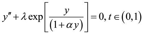
Bratu’s equation [24] was first studied as a simple case of a second-order ordinary differential equation by Bratu [25]. The equation arises when deriving the temperature distribution for a reaction in an infinite vessel with planeparallel walls, and also in a simplification of a combustion reaction with a cylindrical vessel [26]. The differential equation is
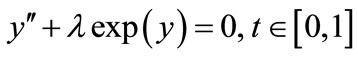 (8)
(8)
with boundary conditions
 (9)
(9)
The analytical solution of Equations (8) and (9) using Homotopy perturbation method (See Appendix A) is
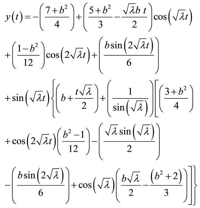 (10)
(10)
where
 (11)
(11)
2.2. Reaction Diffusion Equation and Its Solution
Consider the reaction diffusion equation [16]
 (12)
(12)
with the boundary conditions
 (13)
(13)
The analytical solution of Equations (12) and (13) using Homotopy perturbation method (See Appendix C) is
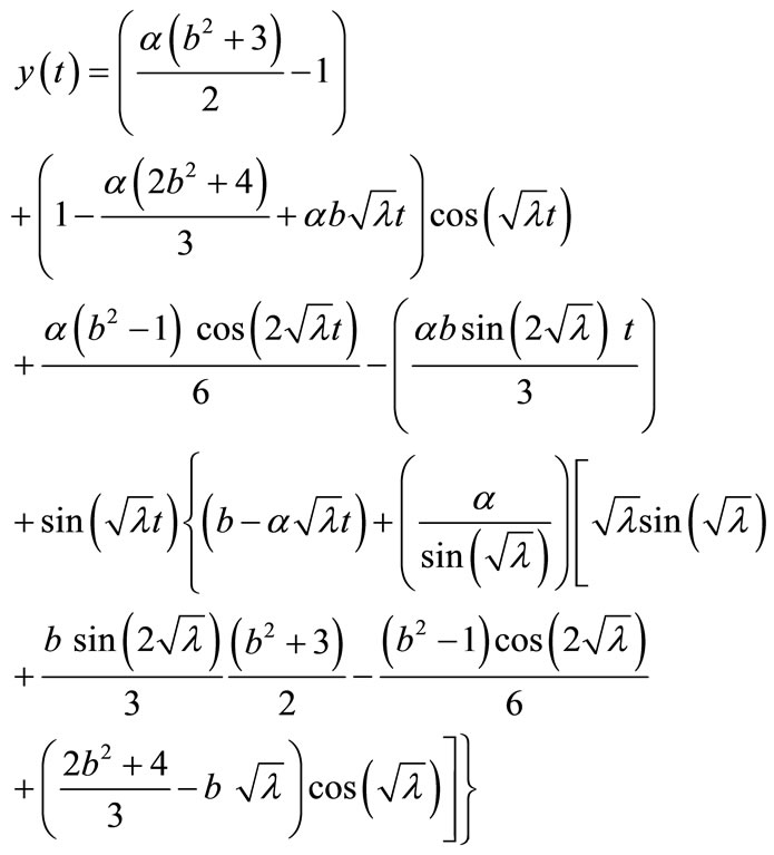 (14)
(14)
where  is defined by Equation (11).
2.3. Troesch’s Problem and Its Solution
Troesch’s problem comes from the investigation of the confinement of a plasma column under radiation pressure. The problem was first described and solved by Weibel [27]. It has become a widely used test problem, and has been solved many times, including in analytical closed form [28] by using a shooting method [29], by using a Laplace transform decomposition technique [30] and most recently by using a modified Homotopy perturbation technique [31]. The differential equation is
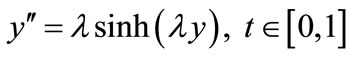 (15)
(15)
with the boundary conditions
 (16)
(16)
The known analytical, closed form solution [28] of Equations (15) and (16) is given by
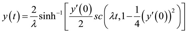 (17)
(17)
where 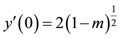 is the derivative at
  and the constant m is the solution to the equation
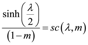 (18)
(18)
We have obtained the analytical solution of Equations (15) and (16) using Homotopy perturbation method (See Appendix F) is
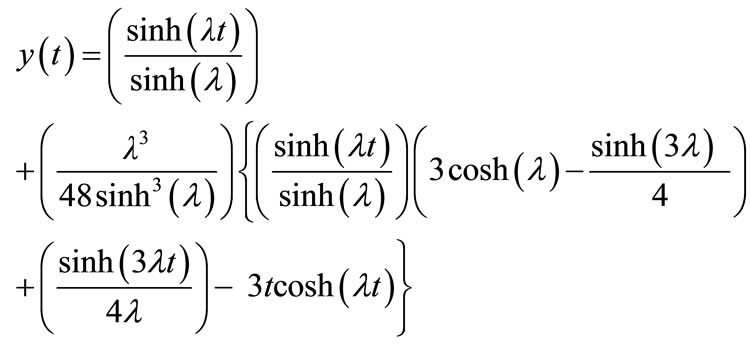 (19)
(19)
2.4. Catalytic Reactions in a Flat Particle and Its Solution
This example arises in a study of heat and mass transfer for a catalytic reaction within a porous catalyst flat particle [32]. The differential equation is the direct result of a material and energy balance. Assuming a flat geometry for the particle and that conductive heat transfer is negligible compared to convective heat transfer yields the differential equation.
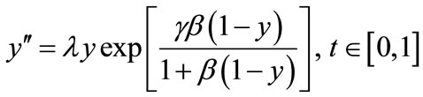 (20)
(20)
with boundary conditions
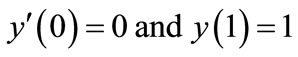 (21)
(21)
The analytical solution of the Equations (20) and (21) using Homotopy perturbation method [33-41] (See Appendix H) is
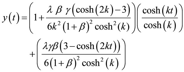 (22)
(22)
where
 (23)
(23)
3. Numerical Simulation
The non-linear equations [Equations (3), (7), (10) and (15)] for the given boundary conditions are solved by numerically. The function pdex4, in Matlab software is used to solve two-point boundary value problems (BVPs) for ordinary differential equations given in Appendix B, Appendix D, Appendix E, Appendix G, Appendix I, Appendix J and Appendix K. The numerical results are also compared with the obtained analytical expressions [Equations (5), (6), (9), (14), (17) and (18)] for all values of parameters ,
,  ,
,  and
and .
.
4. Results and Discussion
Figure 1 represents the dimensionless concentration  versus the dimensionless distance t for different values of the dimensionless parameter
 . From this figure, it is evident that the values of the dimensionless concentration
  increases when dimensionless parameter
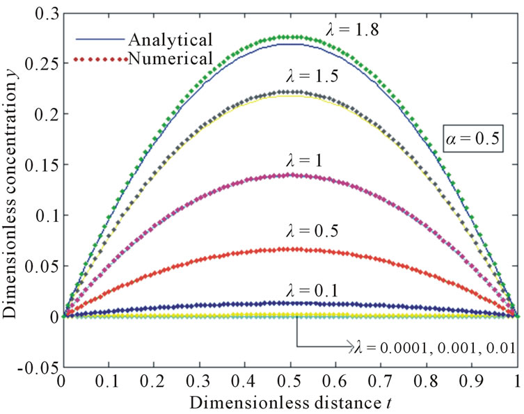
  increases. Figures 2(a)-(d) show the concentration
  versus dimensionless distance t for various values of dimensionless parameters
  and
and . From these figures, it is obvious that the values of the dimensionless concentration
 increases when dimensionless parameters
  increases for the fixed values of
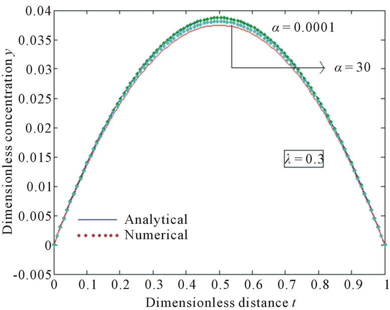
 . From the Figures 3(a) and (b), it is clear that the concentration
  decreases for the different values of the dimensionless parameter
 , for the various values of
 . The dimensionless concentration
 versus the dimensionless distance t for different values of dimensionless parameter
  is plotted in Figure 4.
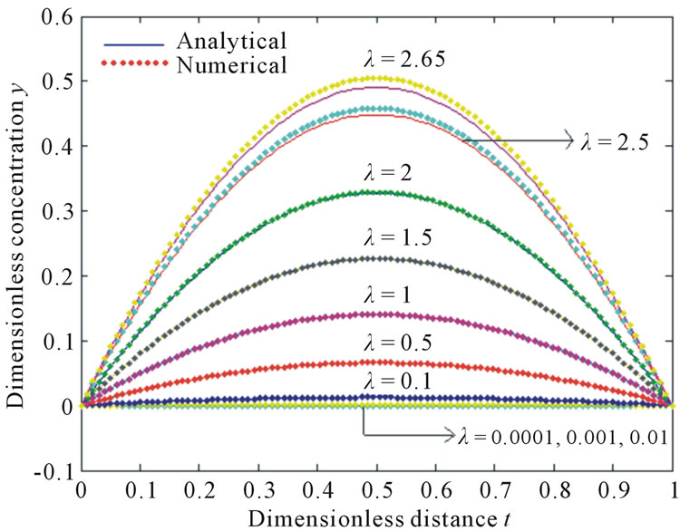
Figure 1. The curve is plotted for the influence of λ on the dimensionless on concentration y(t) versus the dimensionless distance t obtained from the Equations (10) and (11).
 (a)
(a)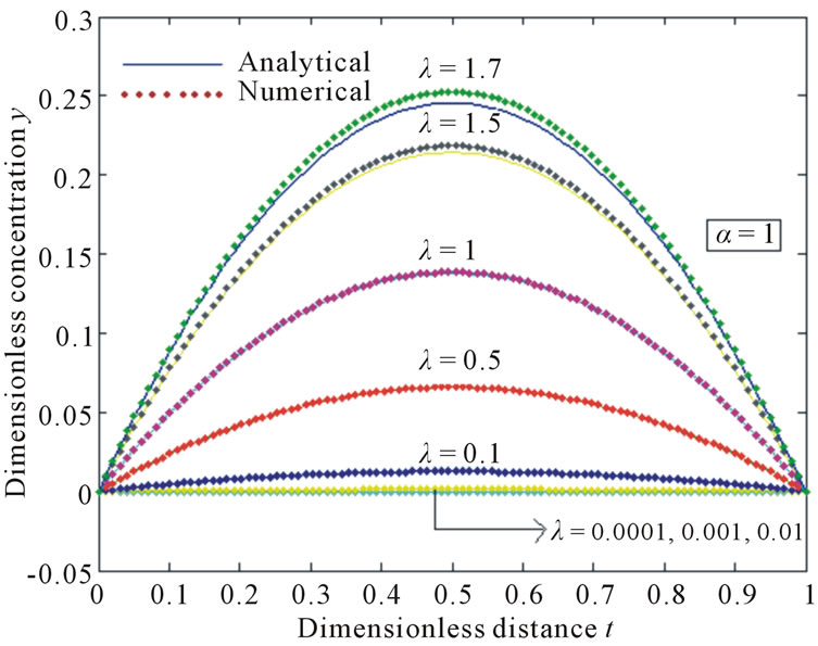 (b)
(b)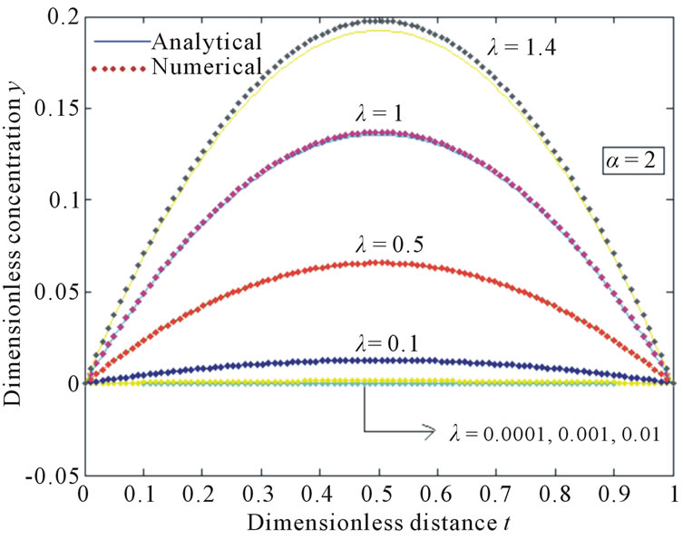 (c)
(c)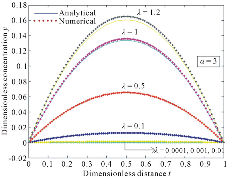 (d)
(d)
Figure 2. Influence of λ on the dimensionless concentration y(t) obtained from the Equation (14). The curve is plotted, when (a) α = 0.5; (b) α = 1; (c) α = 2; (d) α = 3.
 (a)
(a)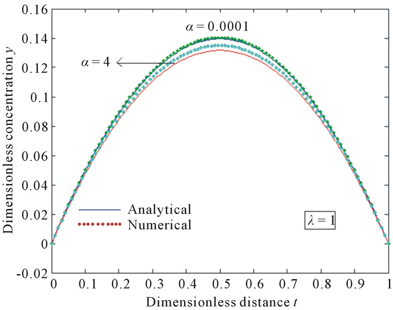 (b)
(b)
Figure 3. Influence of α on the dimensionless concentration y(t) obtained from the Equation (14). The curve is plotted, when (a) λ = 0.3; (b) λ = 1.

Figure 4. The curve is plotted for the influence of λ on the dimensionless concentration y(t) versus the dimensionless distance t from the Equation (19).
From this figure, it shows that the concentration  decreases for the various values of
 . Figures 5(a)-(d) shows the dimensionless concentration
  in the reactor versus the dimensionless distance down the reactor t. From these figures it is clear that the concentration
  decreases for the fixed values of
  and
and  for the different values of
 .
.
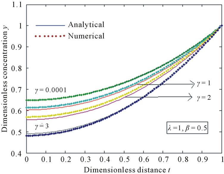
Figures 6 and 7 shows the dimensionless concentration  versus the dimensionless distance t. From these figures it is clear that the concentration
  decreases for the fixed values of
  and
and  for the different values of
 .
.
5. Conclusion
The steady state non-linear reaction-diffusion equation has been solved analytically and numerically. The dimensionless concentrations  in the reactor at the position t are derived by using the HPM. The primary result of this work is simple approximate calculations of concentration for all values of dimensionless parameters
 ,
,  ,
,  and
and . The HPM is an extremely simple method and it is also a promising method to solve other non-linear equations. This method can be easily extended to find the solution of all other non-linear equations.
6. Acknowledgements
This work was supported by the University Grants Commission (F. No. 39-58/2010(SR)), New Delhi, India. The authors are thankful to Mr. M. S. Meenakshisundaram, The Secretary, Dr. R. Murali, The Principal and Dr.
 (a)
(a)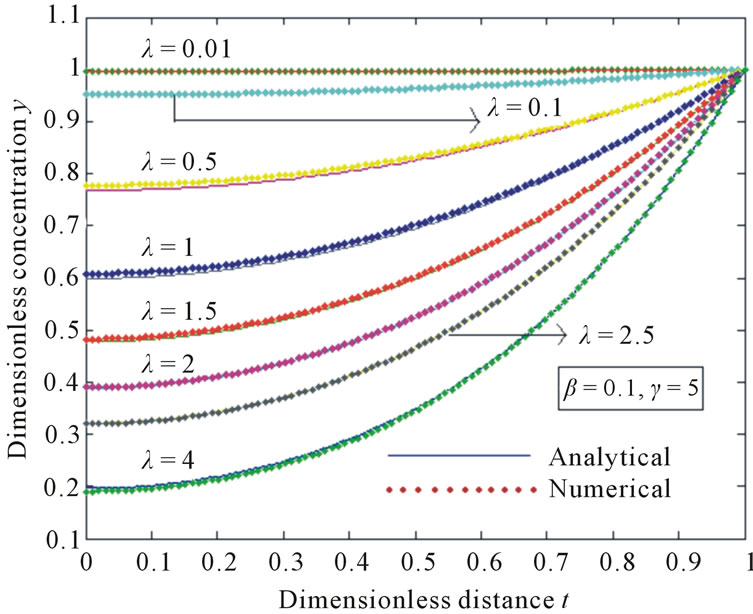 (b)
(b)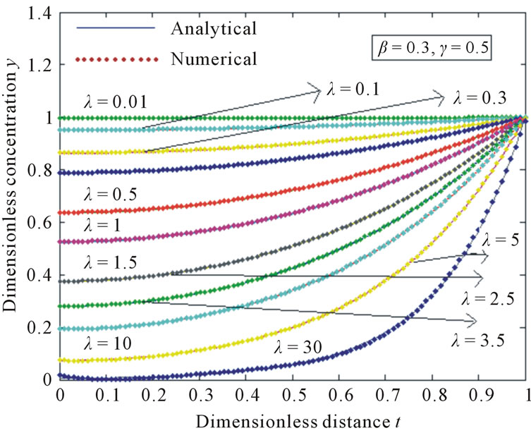 (c)
(c) (d)
(d)
Figure 5. The curve is plotted for the influence of λ on the dimensionless concentration y versus the dimensionless distance down the reactor t obtained from Equations (22) and (23), when (a) β = 0.2, γ = 1; (b) β = 0.1, γ = 5; (c) β = 0.05, γ = 20; (d) β = 0.3, γ = 0.5.
 (a)
(a)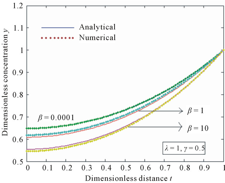 (b)
(b) (c)
(c)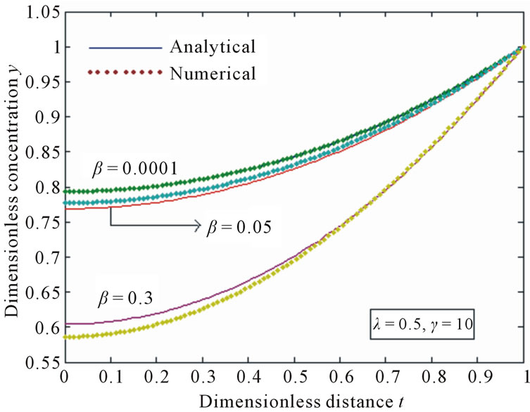 (d)
(d)
Figure 6. The curve is plotted for the influence of β on the dimensionless concentration y versus the dimensionless distance down the reactor t obtained from Equations (22) and (23), when (a) λ = 1, γ = 10; (b) λ = 1, γ = 0.5; (c) λ = 1, γ = 1; (d) λ = 0.5, γ = 10.
 (a)
(a)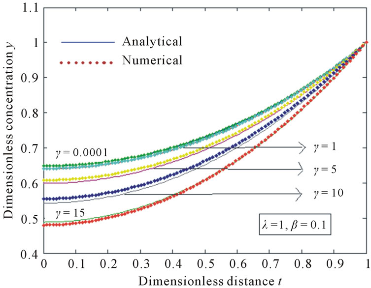 (b)
(b)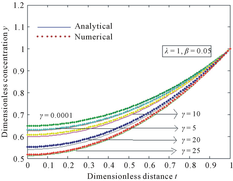 (c)
(c)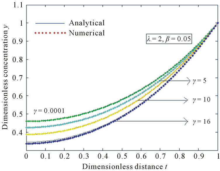 (d)
(d)
Figure 7. The curve is plotted for the influence of γ on the dimensionless concentration y versus the dimensionless distance down the reactor t obtained from Equations (22) and (23), when (a) λ = 1, β = 0.5; (b) λ = 1, β = 0.1; (c) λ = 1, β = 0.05; (d) λ = 2, β = 0.05.
L. Rajendran, Assistant Professor, Department of Mathematics, The Madura College, Madurai for their encouragement.
REFERENCES
- Y. Lin, J. A. Enszer and M. Stadtherr, “Enclosing All Solutions of Two Point Boundary Value Problems for ODEs,” Computers and Chemical Engineering, Vol. 32, 2008, pp. 1714-1725. doi:10.1016/j.compchemeng.2007.08.013
- J. Newman and W. Tiedmann, “Porous-Electrode Theory with Battery Applications,” AIChE Journal, Vol. 21, No. 1, 1975, pp. 25-41. doi:10.1002/aic.690210103
- S. H. Mirmoradi, I. Hosseinpour, S. Ghanbarpour and A. Barari, “Application of an Approximate Analytical Method to Nonlinear Troesch’s Problem,” Applied Mathematical Sciences, Vol. 3, No. 32, 2009, pp. 1579-1585.
- A. Barari, A. R. Ghotbi, F. Farrokhzad and D. D. Ganji, “Variational Iteration Method and Homotopy-Perturbation Method for Solving Different Types of Wave Equations,” Journal of Applied Sciences, Vol. 8, 2008, pp. 120-126. doi:10.3923/jas.2008.120.126
- R. Abdoul, A. Ghotbi, A. Barari and D. D. Ganji, “Solving Ratio-Dependent Redator-Prey System with Constant Effort Harvesting Using Homotopy Perturbation Method,” Journal of Mathematical Problems in Engineering, 2008, Article ID: 945420.
- A. Barari, A. Janalizadeh and D. D. Ganji, “Application of Homotopy Perturbation Method to Zakharov-Kuznetsov Equation,” Journal of Physics, Vol. 96, 2008, pp. 1-8. doi:10.1088/1742-6596/96/1/012082
- A. Barari, D. D. Ganji and M. J. Hosseini, “HomotopyPerturbation Method for a Nonlinear Cerebral ReactionDiffusion Equation,” Arab Journal of Mathematics and Mathematical Sciences, Vol. 1, 2007, pp. 1-9.
- A. Barari, M. Omidvar, A. R. Ghotbi and D. D. Ganji, “Application of Homotopy-Perturbation Method and Variational Iteration Method to Nonlinear Oscillator Differential Equations,” Acta Applicanda Mathematicae, Vol. 104, 2008, pp. 161-171. doi:10.1007/s10440-008-9248-9
- A. Barari, M. Omidvar, D. D. Ganji and Abbas Tahmasebi poor, “An Approximate Solution for Boundary Value Problems in Structural Engineering and Fluid Mechanics,” Journal of Mathematical Problems in Engineering, 2008, Article ID: 394103.
- L. N. Zhang and J. H. He, “Homotopy-Perturbation Method for the Solution of the Electrostatic Potential Differential Equation,” Mathematical Problems in Engineering, 2006, Article ID: 83878. doi:10.1155/MPE/2006/83878
- J. H. He, “New Interpretation of Homotopy-Perturbation Method,” International Journal of Modern Physics B, Vol. 20, No. 18, 2006, pp. 256-2568. doi:10.1142/S0217979206034819
- J.-H. He, “Homotopy-Perturbation Technique,” Computer Methods in Applied Mechanics and Engineering, Vol. 178, No. 3-4, 1999, pp. 257-262. doi:10.1016/S0045-7825(99)00018-3
- J.-H. He, “Homotopy-Perturbation Method: A New NonLinear Analytical Technique,” Applied Mathematics and Computation, Vol. 135, No. 1, 2003, pp. 73-79. doi:10.1016/S0096-3003(01)00312-5
- Y. Chen, “Dynamic System Optimization,” Ph.D. Thesis, University of California, Los Angeles, 2006.
- Y. Chen and V. Manousiouthakis, “Identification of All Solutions of TPBV Problems,” AIChE Annual Meeting, Cincinnati, Dover, New York, 2005.
- M. I. Syam and E. M. Allon, “On the Computations of Fold Points for Non Linear Elliptic Eigen Value Problems,” International Journal of Open Problems in Computer Science and Mathematics, Vol. 4, No. 1, 2011.
- J. P. Abbott, “An Efficient Algorithm for the Determination of Certain Bifurcation Point,” Journal of Computational and Applied Mathematics, Vol. 4, No. 1, 1978, pp. 19-27. doi:10.1016/0771-050X(78)90015-3
- H. Amann, “Fixed Point Equations and Nonlinear Eigenvalue Problems in Ordered Banach Space,” SIAM Review, Vol. 8, 1978, pp. 19-27.
- H. B. Keller and D. S. Choen, “Some Positone Problems Suggested by Nonlinear Heat Generation,” Journal of Mathematics and Mechanics, Vol. 16, 1967, pp. 1361- 1376.
- U. M. Assher, R. M. Matthij and R. D. Russell, “Numerical Solution of Boundary Value Problems for Ordinary Differential Equations,” Society for Industrial and Applied Mathematics, Philadelphia, 1995.
- G. Moore and A. Spence, “The Calculation of Turning Points of Nonlinear Equations,” SIAM Journal on Numerical Analysis, Vol. 17, No. 4, 1980, pp. 567-576. doi:10.1137/0717048
- E. Deeba, S. A. Khuri and S. Xie, “An Algorithm for Solving Boundary Value Problems,” Journal of Computational Physics, Vol. 159, No. 2, 2000, pp. 125-138. doi:10.1006/jcph.2000.6452
- J. B. Rosen, “Approximate Solution and Error Bounds for Quasilinear Elliptic Boundary Value Problems,” SIAM Journal on Numerical Analysis, Vol. 7, No. 1, 1970, pp. 80-103. doi:10.1137/0707004
- H. Davis, “Introduction to Nonlinear Differential and Integral Equations,” Dover, New York, 1962.
- G. Bratu, “Sur Certaines Equations Integrals Non Lineares,” Comptes Rendus, Vol. 150, 1910, pp. 896-899.
- D. A. Frank-Kamenetskii, “Diffusion and Heat Transfer in Chemical Kinetics,” Plenum Press, New York, 1969.
- E. S. Weibel, “Confident of a Plasma Column by Radiation Pressure,” In: R. K. M. Landshoff, Ed., The Plasma in a Magnetic Field, Stanford University Press, Stanford, 1958, pp. 60-76.
- S. M. Roberts and J. Shipman, “On the Closed Form Solution of Troesch’s Problem,” Journal of Computational Physics, Vol. 21, No. 3, 1976, pp. 291-304. doi:10.1016/0021-9991(76)90026-7
- B. A. Troesch, “A Simple Approach to a Sensitive TwoPoint Boundary Value Problem,” Journal of Computational Physics, Vol. 21, No. 3, 1976, pp. 279-290. doi:10.1016/0021-9991(76)90025-5
- S. A. Khuri, “A Numerical Algorithm for Solving Troesch’s Problem,” International Journal of Computer Mathematics, Vol. 80, No. 4, 2003, pp. 493-498. doi:10.1080/0020716022000009228
- X. Feng, L. Mei and G. He, “An Efficient Algorithm for Solving Troesch’s Problem,” Applied Mathematics and Computation, Vol. 189, No. 1, 2007, pp. 500-507. doi:10.1016/j.amc.2006.11.161
- V. Hlavacek, M. Marek and M. Kubicek, “Modelling of Chemical Reactors, X: Multiple Solutions of Enthalpy and Mass Balance for a Catalytic Reaction within a Porous Catalyst Particle,” Chemical Engineering Science, Vol. 23, No. 9, 1968, pp. 1083-1097. doi:10.1016/0009-2509(68)87093-9
- J. H. He, “Homotopy Perturbation Technique,” Computer Methods in Applied Mechanics and Engineering, Vol. 178, No. 3-4, 1999, pp. 257-262. doi:10.1016/S0045-7825(99)00018-3
- J. H. He, “Homotopy Perturbation Method: A New Nonlinear Analytical Technique,” Applied Mathematics and Computation, Vol. 135, No. 1, 2003, pp. 73-79. doi:10.1016/S0096-3003(01)00312-5
- J. H. He, “A Simple Perturbation Approach to Blasius Equation,” Applied Mathematics and Computation, Vol. 140, No. 2-3, 2003, pp. 217-222. doi:10.1016/S0096-3003(02)00189-3
- P. D. Ariel, “Alternative Approaches to Construction of Homotopy-Perturbation Algorithms,” Nonlinear Science Letters A, Vol. 1, 2010, pp. 43-52.
- V. Ananthaswmy, A. Eswari and L. Rajendran, “Analytical Solution of System of Nonlinear Reaction-Diffusion Equations in a Thin Membrane: Homotopy-Perturbation Approach,” Journal of Physical Chmistry, Vol. 5, No. 2, 2010.
- S. Loghambal and L. Rajendran, “Mathematical Modeling of Diffusion and Kinetics of Amperometric Immobilized Enzyme Electrodes,” Electrochim Acta, Vol. 55, No. 18, 2010, pp. 5230-5238. doi:10.1016/j.electacta.2010.04.050
- A. Meena and L. Rajendran, “Mathematical Modeling of Amperometric and Potentiometric Biosensors and System of Non-Linear Equations, Homotopy-Perturbation Approach,” Journal of Electroanalytical Chemistry, Vol. 644, No. 1, 2010, pp. 50-59. doi:10.1016/j.jelechem.2010.03.027
- S. Anitha, A. Subbiah, S. Subramaniam and L. Rajendran, “Analytical Solution of Amperometric Enzymatic Reactions Based on Homotopy-Perturbation Method,” Electrochimica Acta, Vol. 56, No. 9, 2011, pp. 3345-3352. doi:10.1016/j.electacta.2011.01.014
- V. Ananthaswamy and L. Rajendran, “Analytical Solution of Two-Point Non Linear Boundary Value Problems in a Porous Catalyst Particles,” International Journal of Mathematical Archive, Vol. 3, No. 3, 2012, pp. 810-821.
Appendix A: Solution of Bratu’s Equation Using HPM
In this Appendix, we indicate how the Equation (10) is derived. When y is small, Equation (8) is reduces to
 (A1)
(A1)
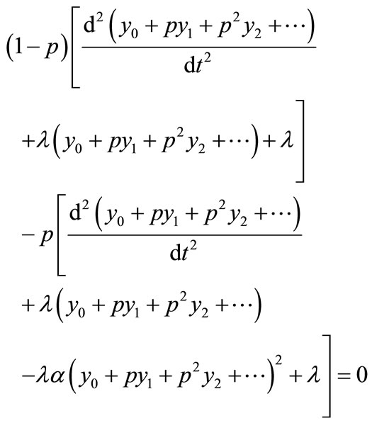
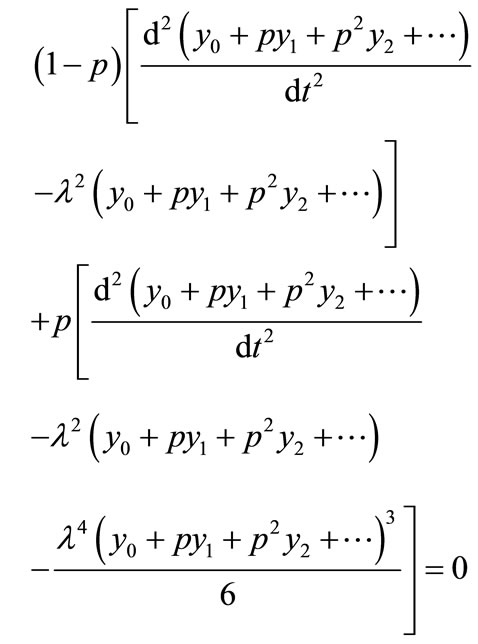
We construct the Homotopy for the Equation (A1) is as follows:
 (A2)
(A2)
The analytical solution of Equation (8) with Equation (9) is
 (A3)
(A3)
Substituting the Equation (A3) into an Equation (A2) we get
 (A4)
(A4)
Comparing the coefficients of like powers of p in Equation (A4) we get
 (A5)
(A5)
 (A6)
(A6)
The initial approximations are as follows
 (A7)
(A7)
 (A8)
(A8)
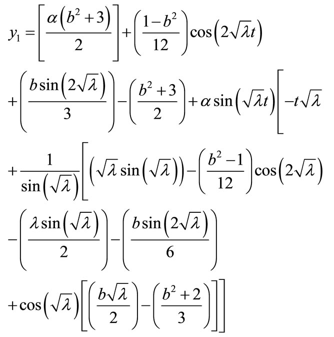
Solving the Equation (A5) and the Equation (A6) and using the boundary conditions Equation (A7) and the Equation (A8) we obtain the following results:
 (A9)
(A9)
 (A10)
(A10)
where b is defined in Equation (9). According to the HPM, we can conclude that
 (A11)
(A11)
After putting the Equation (A9) and Equation (A10) into an Equation (A11) we obtain the solution in the text.
Appendix B: Matlab Program Is to Find the Numerical Solution of the Non Linear Differential Equations (8) and (9)
function pdex4 m = 0;
x = linspace(0,1);
t=linspace(0,10000);
sol= pdepe(m,@pdex4pde,@pdex4ic,@pdex4bc,x,t);
u1 = sol(:,:,1);
figure plot(x,u1(end,:))
title('u1(x,t)')
xlabel('Distance x')
ylabel('u1(x,2)')
%-----------------------------------------------------------------
function [c,f,s] = pdex4pde(x,t,u,DuDx)
c = 1;
f = DuDx;
lamda=2;
F =lamda*exp(u)
s = F;
%-----------------------------------------------------------------
function u0 = pdex4ic(x); %create a initial conditions u0 = 1;
%-----------------------------------------------------------------
function[pl,ql,pr,qr]=pdex4bc(xl,ul,xr,ur,t) %create a boundary conditions pl = ul;
ql = 0;
pr = ur-0;
qr = 0;
Appendix C: Solution of Reaction Diffusion Equation Using HPM
In this Appendix, we indicate how Equation (14) is derived. When  is small, Equation (12) is reduces to
 (C1)
(C1)
We construct the Homotopy for Equation (C1) is as follows:
 (C2)
(C2)
The analytical solution of Equation (12) with Equation (13) is
 (C3)
(C3)
Substituting Equation (C3) into an Equation (C2) we get
 (C4)
(C4)
Comparing the coefficients of like powers of p in Equation (C4) we get
 (C5)
(C5)
 (C6)
(C6)
The initial approximations are as follows:
 (C7)
(C7)
 (C8)
(C8)
Solving the Equations (C5) and (C6) and using the boundary conditions Equation (C7) and the Equation (C8) we obtain the following results:
 (C9)
(C9)
 (C10)
(C10)
where b is defined in the text Equation (6). According to the HPM, we can conclude that
 (C11)
(C11)
After putting Equation (C9) and Equation (C10) into an Equation (C11) we obtain the solution in the text.
Appendix D: Matlab Program Is to Find the Numerical Solution of the Non-Linear Differential Equations (12) and (13)
function pdex4 m = 0;
x = linspace(0,1);
t=linspace(0,10000);
sol= pdepe(m,@pdex4pde,@pdex4ic,@pdex4bc,x,t);
u1 = sol(:,:,1);
figure plot(x,u1(end,:))
title('u1(x,t)')
xlabel('Distance x')
ylabel('u1(x,2)')
%-----------------------------------------------------------------
function [c,f,s] = pdex4pde(x,t,u,DuDx)
c = 1;
f = DuDx;
lamda=1.5;
alpha=0.5;
F =lamda*exp(u/(1+(alpha*u)));
s = F;
%-----------------------------------------------------------------
function u0 = pdex4ic(x); %create a initial conditions u0 = 1;
%-----------------------------------------------------------------
function[pl,ql,pr,qr]=pdex4bc(xl,ul,xr,ur,t) %create a boundary conditions pl = ul;
ql = 0;
pr = ur-0;
qr = 0;
Appendix E: Matlab Program Is to Find the Numerical Solution of the Non Linear Differential Equations (12) and (13)
function pdex4 m = 0;
x = linspace(0,1);
t=linspace(0,10000);
sol= pdepe(m,@pdex4pde,@pdex4ic,@pdex4bc,x,t);
u1 = sol(:,:,1);
figure plot(x,u1(end,J)
title(‘u1(x,t)’)
xlabel(‘Distance x’)
ylabel(‘u1(x,2)’)
%-----------------------------------------------------------------
function [c,f,s] = pdex4pde(x,t,u,DuDx)
c = 1;
f = DuDx;
lamda=0.3;
alpha=30;
F =lamda*exp(u/(1+(alpha*u)));
s = F;
%-----------------------------------------------------------------
function u0 = pdex4ic(x); %create a initial conditions u0 = 1;
%-----------------------------------------------------------------
function[pl,ql,pr,qr]=pdex4bc(xl,ul,xr,ur,t) %create a boundary conditions pl = ul;
ql = 0;
pr = ur-0;
qr = 0;
Appendix F: Solution of Troesch’s Problem Using HPM
In this Appendix, we indicate how the Equation (19) is derived.
When  is small, Equation (15) is reduces to
 (E1)
(E1)
We construct the Homotopy for the Equation (E1) is as follows:
 (E2)
(E2)
The analytical solution of Equation (15) with Equation (16) is
 (E3)
(E3)
Substituting the Equation (E3) into an Equation (E2) we get
 (E4)
(E4)
Comparing the coefficients of like powers of p in Equation (E4) we get
 (E5)
(E5)
 (E6)
(E6)
The initial approximations are as follows
 (E7)
(E7)
 (E8)
(E8)
Solving the Equation (E5) and the Equation (E6) and using the boundary conditions Equation (E7) and the Equation (E8) we obtain the following results:
 (E9)
(E9)
 (E10)
(E10)
According to the HPM, we can conclude that
 (E11)
(E11)
After putting the Equation (E9) and the Equation (E10) into an Equation (E11) we obtain the solution in the text.
Appendix G: Matlab Program Is to Find the Numerical Solution of the Non Linear Differential Equations (15) and (16)
function pdex4 m = 0;
x = linspace(0,1);
t=linspace(0,10000);
sol= pdepe(m,@pdex4pde,@pdex4ic,@pdex4bc,x,t);
u1 = sol(:,:,1);
figure plot(x,u1(end,:))
title('u1(x,t)')
xlabel('Distance x')
ylabel('u1(x,2)')
%-----------------------------------------------------------------
function [c,f,s] = pdex4pde(x,t,u,DuDx)
c = 1;
f = DuDx;
lamda=2.8;
F =-lamda*(sinh(lamda*u))
s = F;
%-----------------------------------------------------------------
function u0 = pdex4ic(x); %create a initial conditions u0 = 1;
%-----------------------------------------------------------------
function[pl,ql,pr,qr]=pdex4bc(xl,ul,xr,ur,t) %create a boundary conditions pl = ul;
ql = 0;
pr = ur-1;
qr = 0;
Appendix H: Solution of Catalytic Reactions in a Flat Particle Using HPM
In this Appendix, we indicate how the Equation (22) is derived. When  is small, Equation (20) is reduces to
 (H1)
(H1)
We construct the Homotopy for the Equation (H1) is as follows:
 (H2)
(H2)
The analytical solution of Equation (20) with Equation (21) is
 (H3)
(H3)
Substituting the Equation (E3) into an Equation (E2) we get
 (H4)
(H4)
Comparing the coefficients of like powers of p in Equation (H4) we get
 (H5)
(H5)
 (H6)
(H6)
The initial approximations are as follows
 (H7)
(H7)
 (H8)
(H8)
Solving the Equation (H5) and the Equation (H6) and using the boundary conditions Equation (H7) and the Equation (H8) we obtain the following result:
 (H9)
(H9)
 (H10)
(H10)
where k is defined in the text Equation (23).
According to the HPM, we can conclude that
 (H11)
(H11)
After putting the Equation (H9) and the Equation (H10) into an Equation (H11) we obtain the solution in the text.
Appendix I: Matlab Program Is to Find the Numerical Solution of the Non Linear Differential Equations (20) and (21)
function pdex4 m = 0;
x =linspace(0,1);
t=linspace(0,10000);
sol= pdepe(m,@pdex4pde,@pdex4ic,@pdex4bc,x,t);
u1 = sol(:,:,1);
figure plot(x,u1(end,J)
title(‘u1(x,t)’)
xlabel(‘Distance x’)
ylabel(‘u1(x,2)’)
%-----------------------------------------------------------------
function [c,f,s] = pdex4pde(x,t,u,DuDx)
c = 1;
f = DuDx;
lamda=4;
beta=0.1;
gamma=5;
F=-lamda*u*exp(beta*gamma*(1-u)/(1+beta*(1-u)));
s = F;
%-----------------------------------------------------------------
function u0 = pdex4ic(x); %create a initial conditions u0 = 1;
% -------------------------------------------------------------
function[pl,ql,pr,qr]=pdex4bc(xl,ul,xr,ur,t) %create a boundary conditions pl = 0;
ql = 1;
pr = ur(1)-1;
qr = 0;
Appendix J: Matlab Program Is to Find the Numerical Solution of the Non Linear Differential Equations (20) and (21)
function pdex4 m = 0;
x =linspace(0,1);
t=linspace(0,10000);
sol= pdepe(m,@pdex4pde,@pdex4ic,@pdex4bc,x,t);
u1 = sol(:,:,1);
figure plot(x,u1(end,:))
title('u1(x,t)')
xlabel('Distance x')
ylabel('u1(x,2)')
%-----------------------------------------------------------------
function [c,f,s] = pdex4pde(x,t,u,DuDx)
c = 1;
f = DuDx;
lamda=1;
beta=0.15;
gamma=10;
F=-lamda*u*exp(beta*gamma*(1-u)/(1+beta*(1-u)));
s = F;
%-----------------------------------------------------------------
function u0 = pdex4ic(x); %create a initial conditions u0 = 1;
%-----------------------------------------------------------------
function[pl,ql,pr,qr]=pdex4bc(xl,ul,xr,ur,t) %create a boundary conditions pl = 0;
ql = 1;
pr = ur(1)-1;
qr = 0;
Appendix K: Matlab Program Is to Find the Numerical Solution of the Non Linear Differential Equations (20) and (21)
function pdex4 m = 0;
x =linspace(0,1);
t=linspace(0,10000);
sol= pdepe(m,@pdex4pde,@pdex4ic,@pdex4bc,x,t);
u1 = sol(:,:,1);
figure plot(x,u1(end,:))
title('u1(x,t)')
xlabel('Distance x')
ylabel('u1(x,2)')
%-----------------------------------------------------------------
function [c,f,s] = pdex4pde(x,t,u,DuDx)
c = 1;
f = DuDx;
lamda=1;
beta=0.1;
gamma=15;
F=-lamda*u*exp(beta*gamma*(1-u)/(1+beta*(1-u)));
s = F;
%-----------------------------------------------------------------
function u0 = pdex4ic(x); %create a initial conditions u0 = 1;
%-----------------------------------------------------------------
function[pl,ql,pr,qr]=pdex4bc(xl,ul,xr,ur,t) %create a boundary conditions pl = 0;
ql = 1;
pr = ur(1)-1;
qr = 0;
Appendix: L Nomenclature
Symbol Meaning
 Dimensionless distance down the reactor
 Dimensionless concentration in the reactor
 Dimensionless parameter
 Dimensionless parameter
 Dimensionless parameter
 Dimensionless parameter
NOTES
*Corresponding author.