Applied Mathematics
Vol.3 No.8(2012), Article ID:21493,3 pages DOI:10.4236/am.2012.38134
Restricted Three-Body Problem in Cylindrical Coordinates System
1Department of Astronomy, Faculty of Science, King Abdulaziz University, Jeddah, KSA
2Department of Mathematics, Faculty of Science, King Abdulaziz University, Jeddah, KSA
Email: sharaf_adel@hotmail.com, alshaary@hotmail.com
Received June 26, 2012; revised July 26, 2012; accepted August 6, 2012
Keywords: Spatial Restricted Circular Three Body Problem; Regularization
ABSTRACT
In this paper, the equations of motion for spatial restricted circular three body problem will be established using the cylindrical coordinates. Initial value procedure that can be used to compute both the cylindrical and Cartesian coordinates and velocities is also developed.
1. Introduction
Depending on the application, a certain coordinate system may be simpler to use than the Cartesian coordinate system. As an example, a physical problem with spherical symmetry defined in R3 (e.g., motion in the field of a point mass), is usually easier to solve in spherical polar coordinates than in Cartesian coordinates. Also, for instance, in the galactic rotation, cylindrical coordinates are usually adopted, while the spherical coordinates are suitable for the dynamics of globular clusters. In fact, the change of the dependent and/or independent variables for the differential equations of motion becomes of the focal point of researches in space dynamics. Some authors proposed successful methods to change of the dependent and/or independent variables so as to regularize the differential equations of motion. Of these, the method established by Stiefel and Scheifele, in 1971 [1]. Many studies on the applications of these devices for some orbital systems were done for the perturbed two body problem (e.g. [2-5]).
The great success of the these devices in regularizing the equations of motion for the perturbed two body problem ,and on the other hand, the importance of the three body problem in space dynamics (e.g [6]) and in stellar dynamics (e.g [7]), tempted us to develop the corresponding deceives for the three body problem.
The present paper represents the first phase of our studies towards establishing new differential equations for the different forms of the three body problem using some important coordinate systems.
The objective of the present paper, is to establish the equations of motion for spatial restricted circular three body problem in cylindrical coordinates system together with initial value procedure that can be used to compute both the cylindrical and Cartesian coordinates and velocities.
2. The Circular Restricted Three-Body Problem
If two of the bodies, say  and
and  in the three-body problem move in circular, coplanar orbits about their common center of mass and the mass of the third body is too small to affect the motion of the other bodies, the problem of the motion of the third body is called the circular ,restricted ,three body problem. The two revolving bodies are called the primaries, their masses are arbitrary but have such internal mass distributions that they may be considered point masses. The equations of motion of the third body in a dimensionless synodic rotating coordinate
 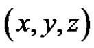 system with the mean motion
 , are [8]
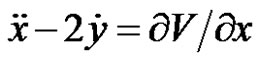 , (1)
, (1)
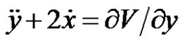 , (2)
, (2)
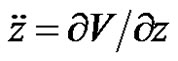 , (3)
, (3)
where  is given as
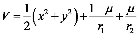 , (4)
, (4)
 denotes the mass of the smaller primary when the total mass of the primaries has been normalized to unity.
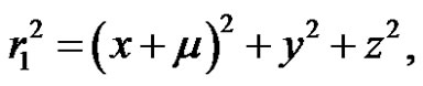 (5)
(5)
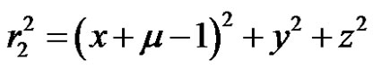 . (6)
. (6)
3. The Equations of Motion in Cylindrical Coordinate System
In what follows we shall establish ,the differential equations for the spatial circular restricted three body problem in the cylindrical coordinate system  together with a list of the direct and the, inverse formulae of the transformation.
3.1. Coordinate and Velocity Transformations
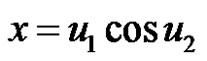 ;
;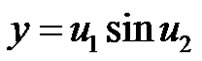 ;
;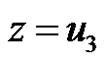 (7)
(7)
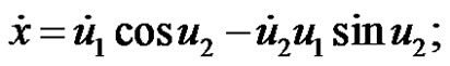
 (8)
(8)
 where
where
 ,
,  ,
, .
.
3.2. Inverse Transformations
From Equation (7) we have
 ;
; ;
; . (9)
. (9)
From Equation (8) we get
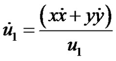 ;
;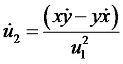 ;
;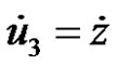 . (10)
where  is given in terms of
 ![]() and y by the first of Equation (9).
and y by the first of Equation (9).
3.3. The Equations of Motion
The kinetic energy of a particle of unit mass in the cylindrical coordinate system is
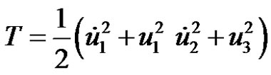 (11)
(11)
By using the transformation equations (Equation (7)), the gravitational potential V could be expressed in term of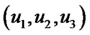 .
.
Using Lagrange’s dynamical equations, we have
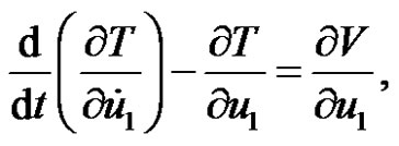
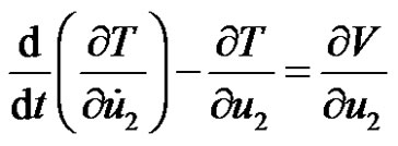 ,
,
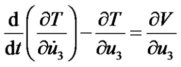 .
.
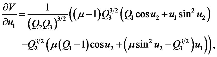
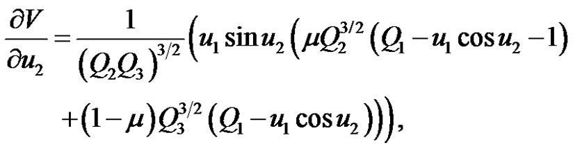
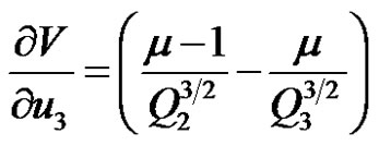
Consequently, we deduce for the equations of motion in the cylindrical coordinate the forms
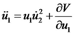 (12.1)
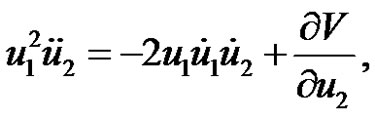 (12.2)
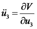 (12.3)
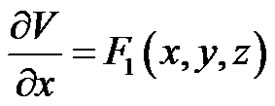
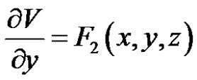
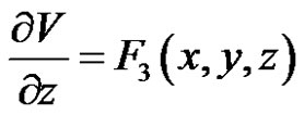
where  are given as
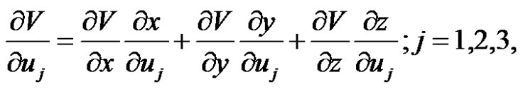 (13)
(13)
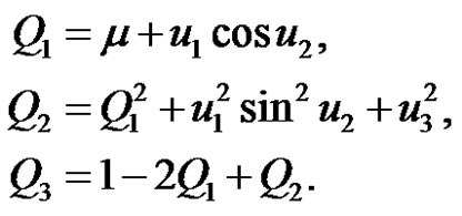
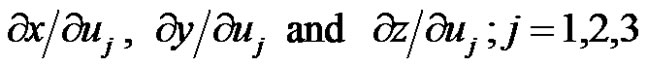 can be computed from Equation (7), while
  and
and  can be computed from Equation (4), and we get
 .
.
where
4. Computational Developments
4.1. Initial Value Procedure
In what follows, we shall establish a procedure that can be used to compute  (say) both:
1) the cylindrical coordinates and velocities
 , and
, and
2) the Cartesian coordinates and velocities
 .
.
So, such procedure is a double usefulness computational algorithm, for which a differential solver can be used for the cylindrical six order system to obtain . While the Cartesian coordinates and velocities
  are obtained by the substitution in the direct transformation formulae (Equations (7) and (8)), rather than solving the six order system of Equations (1), (2) and (3). By this way, great time can be saved.
This initial value procedure using sidereal cylindrical coordinate system will be described through its basic points, input, output and computational steps.
Input: 1)  at
at
2) the final time
3) ,
,  ,
,
 .
.
Output: 1)  from
from ![]() to
to .
.
2)  from
from ![]() to
to .
.
Computational Steps
1) Using the inverse transformation Equations (9) and (10) to find the initial values  using the given values
  at
at .
.
2) Using the partial derivatives  (functions of
 ) to construct the analytical forms of Equation (12) as first order system in the form:
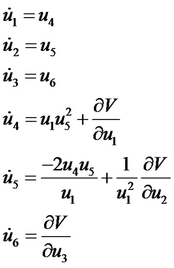
3) Using the initial conditions  from step 1 to solve numerically the above differential system for
  from
from ![]() to
to , (note that
 ).
).
4) Using  from step 3 and the direct transformations Equations (7) and (8) to compute numerically
  and
and 
![]() to
to .
.
5) End.
5. Conclusion
In this paper, the equations of motion for spatial restricted circular three body problem was established in cylindrical coordinates system. Initial value procedure that can be used to compute both the cylindrical and Cartesian coordinates and velocities is also developed.
REFERENCES
- J. Binney and S. Tremaine, “Galactic Dynamics,” Princeton University Press, Princeton, 1987.
- C. D. Murray and S. F. Dermott, “Solar System Dynamics,” Cambridge University Press, Cambridge, 1999.
- M. A. Sharaf, M. R. Arafah and M. E. Awad, “Prediction of Satellites in Earth’s Gravitational Field with Axial Symmetry Using Burdet’s Regularized Theory,” Earth, Moon and Planets, Vol. 38, No. 1, 1987, pp. 21-36. doi:10.1007/BF00115934
- M. A. Sharaf, M. E. Awad and S. A. Najmuldeen, “Motion of Artificial Satellites in the Set of Eulerian Redundant ParametersIII,” Earth, Moon and Planets, Vol. 56, 1992, pp. 141-164.
- M. A. Sharaf and A. A. Sharaf, “Motion of Artificial Earth Satellites in the General Gravity Field Using KS Regularized Theory,” Bulletin of the Faculty of Science, Vol. 63, 1995, pp. 157-181.
- M. A. Sharaf and A. A. Sharaf, “Closest Approach in Universal Variables,” Celestial Mechanics and Dynamical Astronomy, Vol. 69, No. 4, 1998, pp. 331-346. doi:10.1023/A:1008223105130
- E. L. Stiefel and G. Scheifele, “Linear and Regular Celestial Mechanics,” Springer-Verlag, Berlin, 1971.
- V. Szebehely, “Theory of Orbits,” Academic Press, New York, 1967.