Applied Mathematics
Vol. 3 No. 4 (2012) , Article ID: 18890 , 9 pages DOI:10.4236/am.2012.34058
Analytical Expressions of Concentrations inside the Cationic Glucose-Sensitive Membrane
Department of Mathematics, The Madura College, Madurai, India
Email: *raj_sms@rediffmail.com
Received January 31, 2012; revised March 6, 2012; accepted March 13, 2012
Keywords: Homotopy Analysis Method; Cationic Glucose-Sensitive Membrane; Non-Linear Reaction/Diffusion Equations
ABSTRACT
A mathematical model of Wu et al. [J. Membr. Sci 254 (2005) 119-127] of a cationic glucose-sensitive membrane is discussed. The model involves the system of non-linear steady-state reaction-diffusion equations. Analytical expressions pertaining to concentration of oxygen, glucose, and gluconic acid for all values of parameters are presented. We have employed Homotopy analysis method to evaluate the approximate analytical solutions of the non-linear boundary value problem. A comparison of the analytical approximation and numerical simulation is also presented. A good agreement between theoretical predictions and numerical results is observed.
1. Introduction
Diabetes is a chronic disease with major vascular and degenerative complications. The common treatment for diabetic patients is periodic insulin injection. However, poor control of blood glucose level and poor patient compliance are associated with this method. This approach is a poor approximation of normal physiological insulin secretion. The better ways of insulin administration are being sought. Therefore, there is a need for self-regulated delivery systems [1,2] having the capability of adapting the rate of insulin release in response to changes in glucose concentration in order to keep the blood glucose levels within the normal range.
Various sensing mechanisms, such as competitive binding, substrate-enzyme reaction, pH-dependent polymer erosion or drug solubility, and various types of devices, have been applied to design glucose-sensitive insulin delivery systems [3-6]. Horbett and co-workers [7-10] were the first to investigate systems consisting of immobilized glucose oxidase in a pH responsive polymeric hydrogel, enclosing a saturated insulin solution. In insulin delivery system, some of which consist of immobilized glucose oxidase and catalase in pH responsive polymeric hydrogels. According to the nature of charge present, the pH sensitive hydrogels may be classified as cationic or anionic. Cationic glucose sensitive hydrogels were experimentally studied extensively [10-13].
In spite of extensive experimental investigations, only a few studies concerned modelling or theoretical design of such systems [14-17]. Albin et al. [9] developed a mathematical model to describe the steady state behaviour of a cationic glucose-sensitive membrane. Gough and coworkers [15-17] modelled the steady state behaviour and transient response of a cylindrical glucose sensor. Wu et al. [18] derived a mathematical model with consideration of oxygen limitation to describe the glucose sensitivity of a cationic membrane at the steady state.
To our knowledge, no general analytical expressions for the concentration of oxygen, glucose and gluconic acid inside the cationic glucose-sensitive membrane have been reported for all values of the parameters [18]. The purpose of this paper is to derive an analytical expression of the steady-state concentration of reactant by solving the non-linear reaction diffusion equation using Homotopy analysis method (HAM).
2. Mathematical Formulation of the Problem
The reaction scheme in a glucose-sensitive membrane can be written as follows:
 (1)
(1)
The catalase catalyzes the conversion of hydrogen peroxide to oxygen and water:
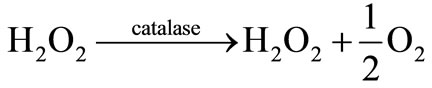 (2)
(2)
If an excess of catalase is immobilized with glucose oxidase, all hydrogen peroxide is reduced. Thus, the overall reaction becomes:
 (3)
(3)
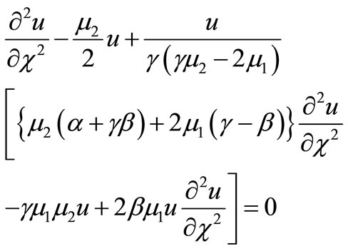
Glucose and oxygen diffuse from the medium into the membrane and glucose is converted to gluconic acid, causing a pH drop and a consequent change in the permeability of the membrane to solutes. Based on the reaction, only one-half of an oxygen molecule is consumed per molecule of glucose when an excess of catalase is present. The corresponding governing non-linear differential equation in planar co-ordinates inside the cationic glucose sensitive membrane may be written as [18]:
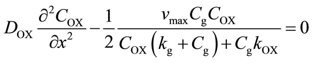 (4)
(4)
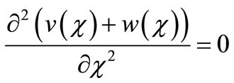
 (5)
(5)
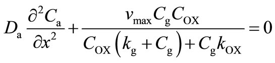 (6)
(6)
where ,
,  and
and  denote the concentration of the oxygen, glucose and gluconic acid respectively.
  are the corresponding diffusion coefficients.
  is the spatial coordinate and
  is the maximum reaction rate.
  are MichaelisMenten constant for the glucose and glucose oxidase respectively. Equations (4)-(6) are solved for the following boundary conditions by assuming that the membrane is immersed in a well stirred external medium with a constant concentration of each species due to continous flow of a fresh medium.
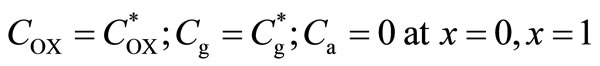 (7)
(7)
where l is the thickness of the membrane and  and
and  are the concentrations of oxygen and glucose in the external solution, respectively. We can assume that the diffusion coefficient of glucose and gluconic acid are equal (
 ). We make the non-linear differenttial Equations (4)-(6) dimensionless form by defining the following dimensionless
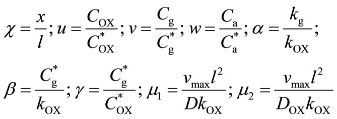 (8)
(8)
Equations (4)-(6) are reduced to the following dimensionless forms:
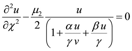 (9)
(9)
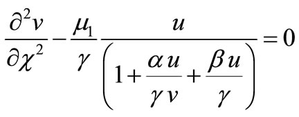 (10)
(10)
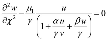 (11)
(11)
where u, v and w represent the dimensionless concentration of oxygen, glucose and gluconic acid.  are dimensionless constant.
  are the Thiele modulus for the oxygen and glucose. Now the boundary conditions reduces to
 (12)
(12)
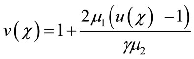
The dimensionless concentration of oxygen , glucose
  and gluconic acid
  are all related processes. On simplifying Equations (9) and (10) we get,
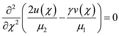 (13)
(13)
Integrating Equation (13), using the boundary conditions (Equation (12)) we get,
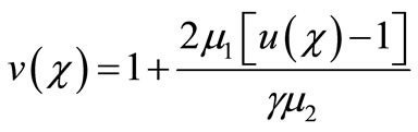 (14)
(14)
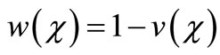
On simplifying Equations (10) and (11) we get,
 (15)
(15)
Integrating Equation (15) and using the boundary conditions (Equation (12)) we get,
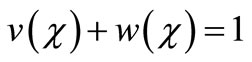 (16)
(16)
So we wish to obtain an analytical expression for the concentration profile  of oxygen. From this concentration profile one can obtain the concentration of glucose
  and gluconic acid
 .
.
3. Approximate Analytical Solutions
3.1. Homotopy Analysis Method (HAM)
The Homotopy analysis method (HAM) [19-22] is a general analytic approach to get series solutions of various types of non-linear equations. More importantly, this method provides us a simple way to ensure the convergence of solution series. The HAM gives us with great freedom to choose proper base functions to approximate a non-linear problem. Since Liao’s book [23] for the Homotopy analysis method was published in 2003, more and more researchers have been successfully applying this method to various non-linear problems [24] in science and engineering. We have solved the non-linear problem using this method. The basic concept of the method is described in Appendix A. Detailed derivation of the dimensionless concentration of oxygen, glucose and gluconic acid are described in Appendix B.
3.2. Solution of Boundary Value Problem
Solution of the system of three non-linear differential equations, (Equations (9)-(11)) with boundary conditions (Equation (12)) give a concentration profile of each species within the membrane.
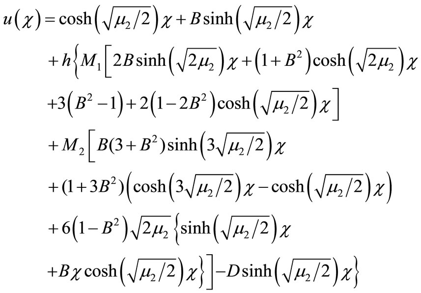 (17)
(17)
 (18)
(18)
 (19)
(19)
where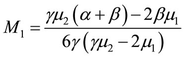 ;
;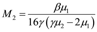 ;
; ;
;
 (20)
(20)
Here h is the convergence control parameter. Equations (17)-(19) represent the analytical expression of the concentration of oxygen , glucose
  and gluconic acid
  respectively.
4. Discussion
The non-linear Equations (9)-(11) are also solved by numerical methods using Scilab/Matlab program. The function pdex4 is used for solving the initial-boundary value problems for parabolic-elliptic partial differential equations. The obtained analytical results are compared with the numerical results for various values of α, β, γ, μ1 and μ2. All possible numerical values of the dimensionless parameters used in Wu et al. [18] and in this work are given in Table 1.
This numerical solution is compared with our analytical results in Figures 1-3 and Table 2. The average relative error between our analytical result (Equation (17)) and the numerical result of oxygen concentration  is less than 0.8% for various values of μ1 and μ2.
The experimental value of the parameters α and β are very small. Since the numerical value of  is 20, the value of
  and
and  becomes very small. In this case the Equation (17) becomes
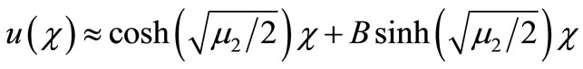 .
.
Figure 1 presents the analytical and numerical concentration profiles of oxygen , glucose
  and gluconic acid
  for the values of the parameters taken in Wu et al. [18].
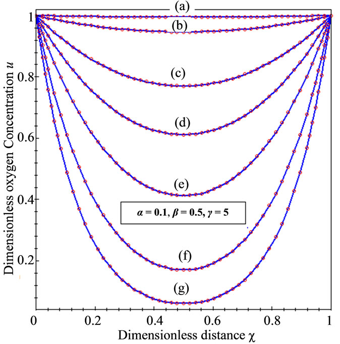
Figures 2 and 3 illustrate the concentration profiles of oxygen u, glucose , and gluconic acid
  for various values of
 . In all the cases the concentration of oxygen
 , glucose
  are decreases and gluconic acid
  increases with the increasing value of parameters
 .
.
The concentration of oxygen and glucose decreases
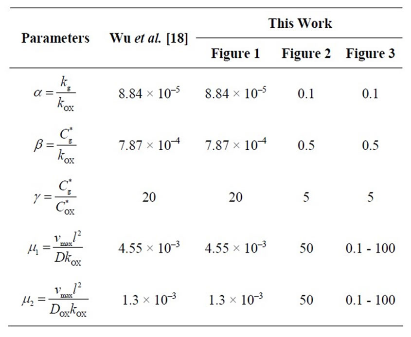
Table 1. Numerical values for dimensionless parameters used in this work. The fixed values of the dimensional parameters used in Wu et al. [18] are kg = 6.187 × 10⁻⁷ mol/cm3, kOX = 6.992 × 10⁻³ mol/cm3,  = 5.5 × 10⁻⁶ mol/cm3,
  = 0.274 × 10⁻⁶ mol/cm3, vmax = 2150 × 10–9 s–1∙mol/cm3, D = 6.75 × 10⁻⁶ cm2/sec DOX = 2.29 × 10⁻⁵ cm2/sec and l = 10–2 cm.
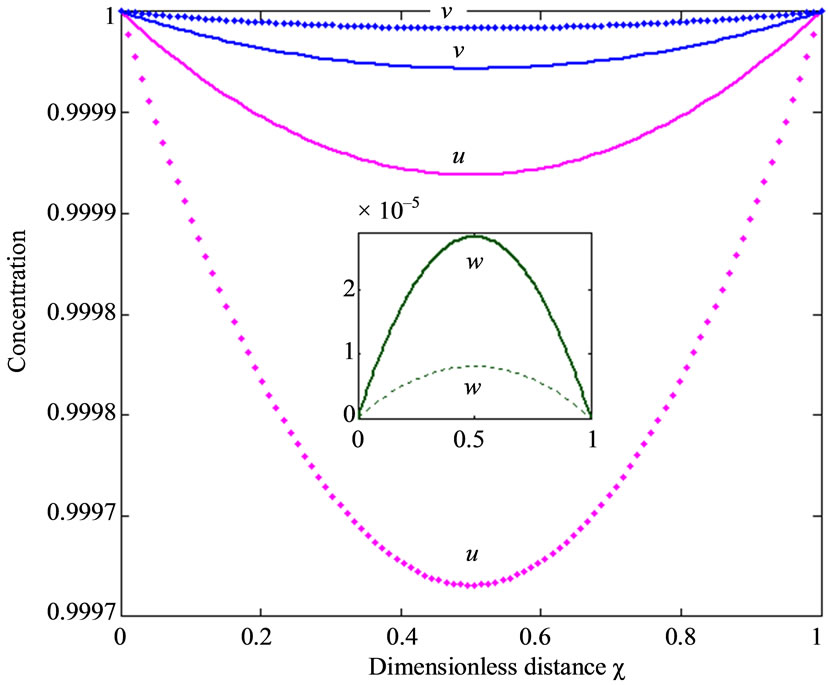
Figure 1. Dimensionless concentration profiles of oxygen u glucose v and gluconic acid w, against the dimensionless distance χ for α = 8.84 × 10⁻⁵, β = 7.87 × 10⁻⁴, γ = 20.07, μ1 = 4.55 × 10⁻³, μ2 = 1.3 × 10⁻³, and h = –0.8. Solid lines represent the analytical solution whereas the dotted lines for the numerical solution.
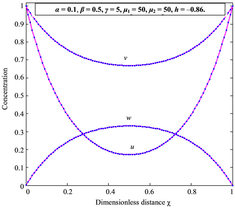
Figure 2. Dimensionless concentration profiles of oxygen u, glucose v, and gluconic acid w against the dimensionless distance χ for α = 0.1, β = 0.5, γ = 5, μ1 = μ2 = 50 and h = –0.86. Solid lines represent the analytical solution whereas the dotted lines for the numerical solution.
within the enzyme matrix from both interfaces ( and
and ), reaching a minimum value at a distance (
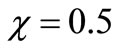 ) within the membrane which is determined by the kinetics of the enzyme reaction and the diffusion properties of the reactants. The concentrations of gluconic acid w increases from both interfaces and reaching a maximum value at the middle of the membrane.
5. Conclusions
A non-linear time independent equation has been solved
 (A)
(A) 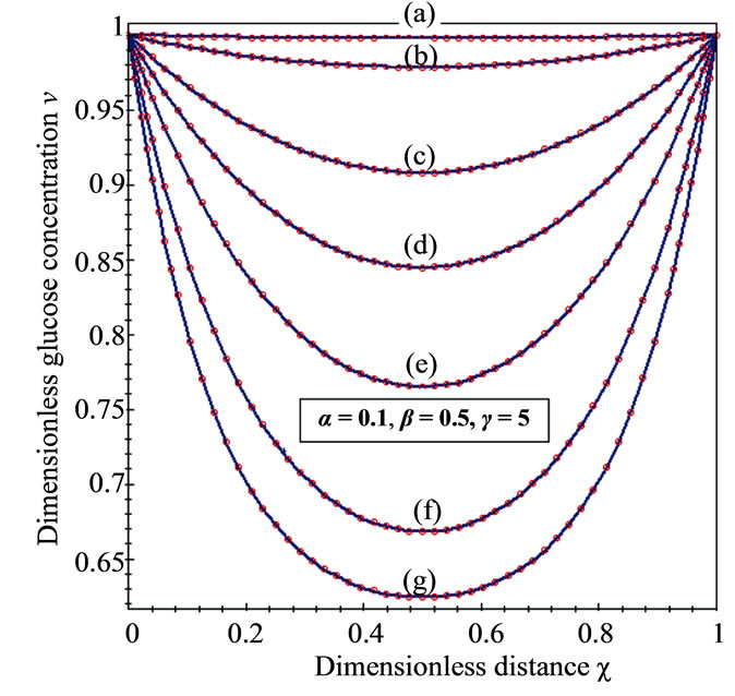 (B)
(B) 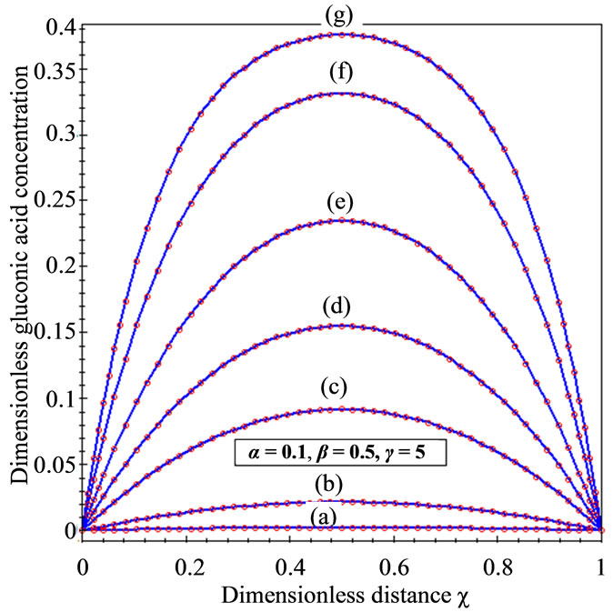 (C)
(C)
Figure 3. Dimensionless concentration profiles of oxygen u (A), glucose v (B), and gluconic acid w (C) against the dimensionless distance χ for (a) μ1 = μ2 = 0.1, h = –0.55; (b) μ1 = μ2 = 1, h = –0.559; (c) μ1 = μ2 = 5, h = –0.62; (d) μ1 = μ2 = 10, h = –0.675; (e) μ1 = μ2 = 20, h = –0.74; (f) μ1 = μ2 = 50, h = –0.8; (g) μ1 = μ2 = 100, h = –0.799.
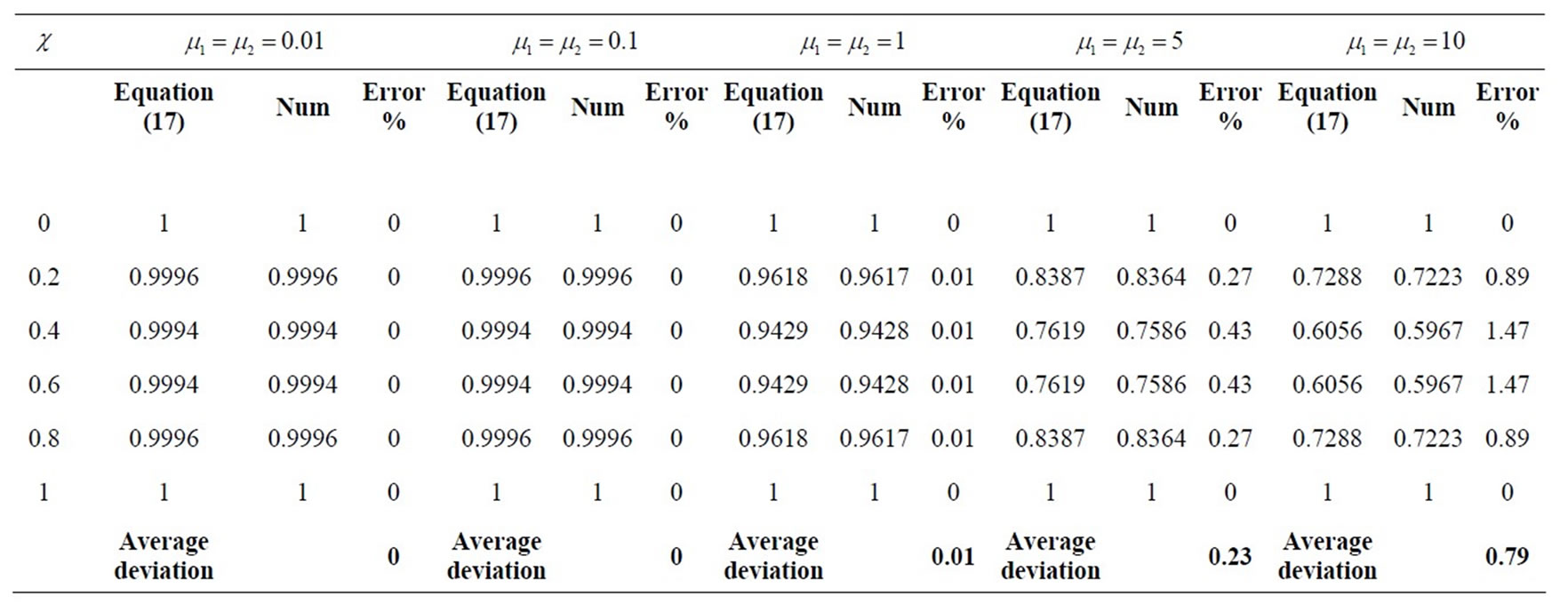
Table 2. Comparison of normalized analytical steady-state concentrations of oxygen u (Equation (17)) with the numerical results for various values of μ1 and μ2 and some fixed values of α = 8.84 × 10⁻⁵, β = 7.78 ×10⁻⁴, and γ = 20 (here h = –0.01).
analytically using homotopy analysis method. The primary result of this work is the first approximate calculations concentrations of oxygen, glucose and gluconic acid for diffusion reaction at the steady state. A simple closed form of analytical expression of concentration of oxygen, glucose and gluconic acid are given in terms of parameters. The analytical results can be used to analyze the effect of different parameters and optimization of the design of glucose membrane.
6. Acknowledgements
This work was supported by the Council of Scientific and Industrial Research (CSIR No. 01(2442)/10/EMR-II), Government of India. The authors also thank Mr. M. S. Meenakshisundaram, Secretary, The Madura College Board, Dr. R. Murali, The Principal, Prof. S. Thiagarajan, H.O.D, Mathematics, The Madura College (Autonomous), Madurai, for their constant encouragement. The authors S. Sevakaperumal and S. Loghambal are very thankful to the Manonmaniam Sundaranar University, Tirunelveli for allowing to do the research work.
REFERENCES
- K. Park, “Nanotechnology: What It Can Do for Drug Delivery,” Journal of Controlled Release, Vol. 120, No. 1-2, 2007, pp. 1-3. doi:10.1016/j.jconrel.2007.05.003
- J. Kost and R. Langer, “Responsive Polymer Systems for Controlled Delivery of Therapeutics,” Trends in Biotechnology, Vol. 10, 1992, pp. 127-131. doi:10.1016/0167-7799(92)90194-Z
- L. A. Klumb and T. A. Horbett, “Design of Insulin Delivery Devices Based on Glucose Sensitive Membranes,” Journal of Controlled Release, Vol. 18, No. 1, 1992, pp. 59-80. doi:10.1016/0168-3659(92)90212-A
- J. Kost and R. Langer, “Responsive Polymeric Delivery Systems,” Advanced Drug Delivery Reviews, Vol. 46, No. 1, 2001, pp. 125-148.
- S. W. Kim and H. A. Jacobs, “Self-Regulated Insulin Delivery-Artificial Pancreas,” Drug Development and Industrial Pharmacy, Vol. 20, No. 4, 1994, pp. 575-580. doi:10.3109/03639049409038319
- S. J. Lee and K. Park, “Glucose-Sensitive Phase-Reversible Hydrogels,” In: R. M. Ottenbrite, S. J. Huang and K. Park, Eds., Hydrogels and Biodegradable Polymers for Bioapplications, ACS, Washington DC, 1996, pp. 11-16.
- J. Kost, T. A. Horbett, B. D. Ratner and M. Singh, “Glucose-Sensitive Membranes Containing Glucose Oxidase: Activity, Swelling, and Permeability Studies,” Journal of Biomedical Materials Research, Vol. 19, No. 9, 1985, pp. 1117-1133. doi:10.1002/jbm.820190920
- G. Albin, T. A. Horbet and B. D. Ratner, “Glucose-Sensitive Membranes for Controlled Delivery of Insulin: Insulin Transport Studies,” Journal of Controlled Release, Vol. 2, No. 3, 1985, pp. 153-164. doi:10.1016/0168-3659(85)90041-0
- G. Albin, T. A. Horbet, S. R. Miller and N. L. Ricker, “Theoretical and Experimental Studies of Glucose Sensitive Membranes,” Journal of Controlled Release, Vol. 6, No. 1, 1987, pp. 267-291. doi:10.1016/0168-3659(87)90081-2
- G. Albin, T. A. Horbett and B. D. Ratner, “Gulcose-Sensitive Membranes for Controlled Delivery of Insulin,” In: J. Kost, Ed., Pulsed and Self-Regulated Drug Delivery, CRC Press, Boca Raton, 1990, pp. 159-185.
- T. Traitel, Y. Cohen and J. Kost, “Characterization of a Glucose Sensitive Insulin Release System in Simulated in Vivo Conditions,” Biomaterials, Vol. 21, No. 16, 2000, pp. 1679-1687. doi:10.1016/S0142-9612(00)00050-8
- M. Glodrich and J. Kost, “Glucose Sensitive Polymeric Matrices for Controlled Drug Delivery,” Clinical Materials, Vol. 13, No. 1-4, 1993, pp. 135-142. doi:10.1016/0267-6605(93)90100-L
- K. Podual, F. J. Doyle III and N. A. Peppas, “Glucose Sensitivity of Glucose Oxidase Containing Cationic Copolymer Hydrogels Having Poly(Ethylene Glycol) Grafts,” Journal of Controlled Release, Vol. 67, No. 1, 2000, pp. 9-17. doi:10.1016/S0168-3659(00)00195-4
- K. Podual, F. J. Doyle III and N. A. Peppas, “Dynamic Behavior of Glucose Oxidase-Containing Microparticles of Poly(Ethylene Glycol)-Grafted Cationic Hydrogels in an Environment of Changing pH,” Biomaterials, Vol. 21, No. 14, 2000, pp.1439-1450. doi:10.1016/S0142-9612(00)00020-X
- J. K. Leypoldt and D. A. Gough, “Model of a Two-Substrate Enzyme Electrode for Glucose,” Analytical Chemistry, Vol. 56, No. 14, 1984, pp. 2896-2904. doi:10.1021/ac00278a063
- D. A. Gough, J. Y. Lusisano and P. H. S. Tse, “Two-Dimensional Enzyme Electrode Sensor for Glucose,” Analytical Chemistry, Vol. 57, No. 12, 1985, pp. 2351-2357. doi:10.1021/ac00289a042
- J. Y. Lusisano and D. A. Gough, “Transient Response of the Two Dimensional Glucose Sensor,” Analytical Chemistry, Vol. 60, No. 13, 1988, pp. 1272-1281. doi:10.1021/ac00164a007
- M. J. Abdekhodaie and X. Y. Wu, “Modeling of a Cationic Glucose-Sensitive Membrane with Consideration of Oxygen Limitation,” Journal of Membrane Science, Vol. 254, No. 1-2, 2005, pp. 119-127.
- S. J. Liao, “The Proposed Homotopy Analysis Technique for the Solution of Nonlinear Problems,” Ph.D. Thesis, Shanghai Jiao Tong University, Shanghai, 1992.
- S. J. Liao, “On the Homotopy Analysis Method for Nonlinear Problems,” Applied Mathematics and Computation, Vol. 147, No. 2, 2004, pp. 499-513. doi:10.1016/S0096-3003(02)00790-7
- S. J. Laio, “Notes on the Homotopy Analysis Method: Some Definitions and Theorems,” Communications in Nonlinear Science and Numerical Simulation, Vol. 14, No. 4, 2009, pp. 983-997. doi:10.1016/j.cnsns.2008.04.013
- S. J. Liao and Y. Tan, “A General Approach to Obtain Series Solutions of Nonlinear Differential Equations,” Studies in Applied Mathematics, Vol. 119, No. 4, 2007, pp. 297-355. doi:10.1111/j.1467-9590.2007.00387.x
- S. J. Liao, “Beyond Perturbation: Introduction to the Homotopy Analysis Method,” Chapman and Hall, CRC Press, Boca Raton, 2003, p. 336.
- S. Loghambal and L. Rajendran, “Analytical Expressions of concentration of Nitrate Pertaining to the Electrocatalytic Reduction of Nitrate Ion,” Journal of Electroanalytical Chemistry, Vol. 661, No. 1, 2011, pp. 137-143. doi:10.1016/j.jelechem.2011.07.027
- G. Domairry and M. Fazeli, “Homotopy Analysis Method to Determine the Fin Efficiency of Convective Straight Fins with Temperature-Dependent Thermal Conductivity,” Communications in Nonlinear Science and Numerical Simulation, Vol.14, No. 2, 2009, pp.489-499. doi:10.1016/j.cnsns.2007.09.007
Appendix A
Basic Idea of Liao’s Homotopy Analysis Method
Basic concept of the Homotopy analysis method is given in the supplementary material of this manuscript.
Appendix B
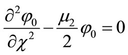
Approximate Analytical Solutions of the Equation (9)
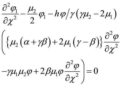
Substituting Equation (14) in Equation (9) and simplifying we get,
 (B1)
(B1)
In order to solve Equation (B1) by means of the HAM, we first construct the zeroth-order deformation equation by taking ,
,
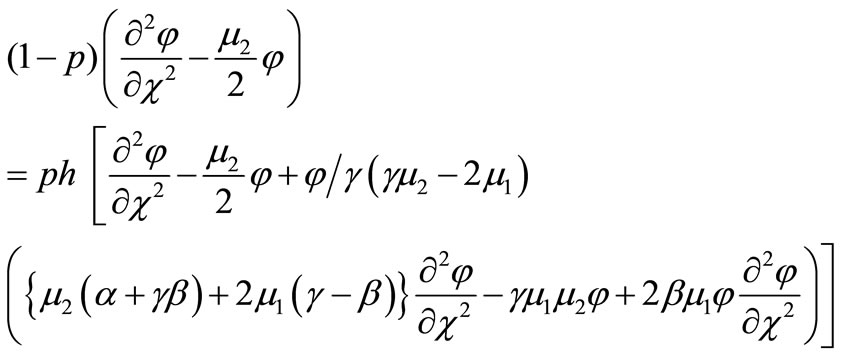 (B2)
(B2)
where  is an embedding parameter. When
 , the above equation becomes,
 (B3)
(B3)
Solving Equation (B3) and using the boundary condition
 and
and  (B4)
(B4)
we get
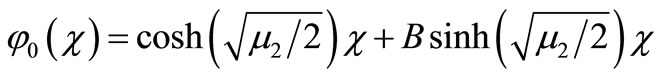 (B5)
(B5)
where 
When  the Equation (B2) is equivalent to Equation (B1), thus it holds.
 (B6)
(B6)
Expanding  in Taylor series with respect to the embedding parameter p, we have,
 (B7)
(B7)
where
 (B8)
(B8)
 (B9)
(B9)
and 
 will be determined later. Note that the above series contains the convergence control parameter h. Assuming that h is chosen so properly that the above series is convergent at
 . We have the solution series as
 (B10)
(B10)
Substituting (B10) into the zeroth-order deformation Equations (B7) and (B8) equating the co-efficient of p we have,
 (B11)
(B11)
Solving Equation (B11) and using the boundary conditions , we get
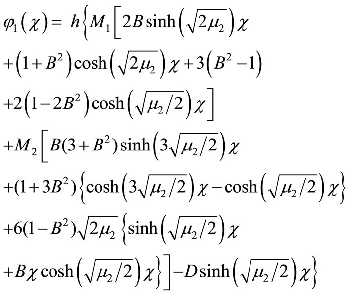 (B12)
(B12)
Adding Equations (B5) and (B12) we obtain the final results as described in Equation (17) in the text.
Appendix C
Scilab/Matlab Program
A SCILAB/MATLAB program for the numerical solution of the system of non-linear second order differential Equations (9)-(11).
Supplementary Material
Appendix A
Basic idea of Liao’s Homotopy Analysis Method
Consider the following differential equation [22]:
 (A1)
(A1)
where, Ν is a nonlinear operator,  denotes an independent variable, u(
 ) is an unknown function. For simplicity, we ignore all boundary or initial conditions, which can be treated in the similar way. By means of generalizing the conventional homotopy method [16], Liao constructed the so-called zero-order deformation equation as:
 (A2)
(A2)
where p [0,1] is the embedding parameter, h ≠ 0 is a nonzero auxiliary parameter, H(
 ) ≠ 0 is an auxiliary function, L is an auxiliary linear operator,
  (
( ) is an initial guess of u(
 ) and
) and  is an unknown function. It is important, that one has great freedom to choose auxiliary unknowns in HAM. Obviously, when
  and
and , it holds:
 and
and  (A3)
(A3)
respectively. Thus, as p increases from 0 to 1, the solution  varies from the initial guess
  to the solution u(
 ). Expanding
  in Taylor series with respect to p, we have:
 (A4)
(A4)
where
 (A5)
(A5)
If the auxiliary linear operator, the initial guess, the auxiliary parameter h, and the auxiliary function are so properly chosen, the series (A4) converges at p = 1 then we have:
 . (A6)
Define the vector
 (A7)
(A7)
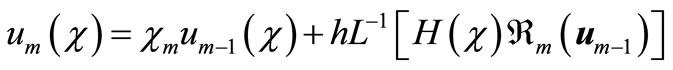
Differentiating Equation (A2) for m times with respect to the embedding parameter p, and then setting p = 0 and finally dividing them by m!, we will have the so-called mth-order deformation equation as:
 (A8)
(A8)
where
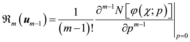 (A9)
(A9)
and
 (A10)
(A10)
Applying  on both side of Equation (A8), we get
 (A11)
(A11)
In this way, it is easily to obtain  for
for  at
at  order, we have
when , we get an accurate approximation of the original equation (A1). For the convergence of the above method we refer the reader to Liao [25]. If Equation (A1) admits unique solution, then this method will produce the unique solution. If Equation (A1) does not possess unique solution, the HAM will give a solution among many other (possible) solutions.
Appendix C
Scilab/Matlab Program
A Scilab/Matlab program for the numerical solution of the system of non-linear second order differential Equations (9)-(11)
function pdex4
m = 0;
x = linspace(0,1);
t = linspace(0,100000);
sol = pdepe(m,@pdex4pde,@pdex4ic,@pdex4bc,x,t);
u1 = sol(:,:,1);
u2 = sol(:,:,2);
u3 = sol(:,:,3);
figure
plot(x,u1(end,:))
title('u1 (x,t)')
xlabel('Distance x')
ylabel('u1 (x,2)')
%--------------------------------------------------------------
figure
plot(x,u2(end,:))
title('u2 (x,t)')
xlabel('Distance x')
ylabel('u2 (x,2)')
% -------------------------------------------------------------
figure
plot(x,u3(end,:))
title('u3 (x,t)')
xlabel('Distance x')
ylabel('u3 (x,2)')
% -------------------------------------------------------------
function [c,f,s] = pdex4pde(x,t,u,DuDx)
c = [1; 1; 1];
f = [1; 1; 1] .* DuDx;
a = 0.5;
b = 5;
y = 5;
u2 = 0.1;
u1 = 5;
F = -u2*u (1)/(2*(a/y*u(1)/u(2)+b/y*u(1)+1));
F1 = -u1*u (1)/(y*(a/y*u(1)/u(2)+b/y*u(1)+1));
F2 = u1*u (1)/(y*(a/y*u(1)/u(2)+b/y*u(1)+1));
S = [F; F1; F2];
% -------------------------------------------------------------
function u0 = pdex4ic(x);
u0 = [0; 1; 0];
% -------------------------------------------------------------
function [pl,ql,pr,qr]=pdex4bc(xl,ul,xr,ur,t)
pl = [ul(1)-1; ul(2)-1; ul(3)];
ql = [0; 0; 0];
pr = [ur(1)-1; ur(2)-1; ur(3)];
qr = [0; 0; 0];
NOTES
*Corresponding author.