Applied Mathematics
Vol. 3 No. 3 (2012) , Article ID: 18108 , 7 pages DOI:10.4236/am.2012.33043
A Direct Derivation of the Exact Fisher Information Matrix for Bivariate Bessel Distribution of Type I
1Department of Statistics, Fasa University, Fasa, Iran
2Department of Statistics, College of Sciences, Shiraz University, Shiraz, Iran
Email: kazemimr88@gmail.com, nematollahi@susc.ac.ir
Received December 10, 2011; revised February 6, 2012; accepted February 14, 2012
Keywords: Bessel Distribution; Fisher Information Matrix; Digamma Function
ABSTRACT
This paper deals with a direct derivation of Fisher’s information matrix for bivariate Bessel distribution of type I. Some tools for the numerical computation and some tabulations of the Fisher’s information matrix are provided.
1. Introduction
The role of the Bessel functions in probability distributions can be trace back to [1,2]. The application of the univariate Bessel distribution in creating a robust alternative to the normal distribution is investigated by [3]. Univariate Bessel function distributions have been also used to the signal processing, [4]. Basic properties of these distributions with their links with some well-known distributions are described in [5]. More discussion on Bessel Distributions can be found in [6]. The bivariate Bessel distribution of type one (BB1) is specified by the following joint density function
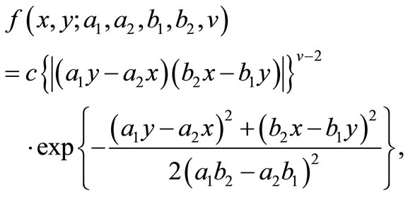 (1.1)
(1.1)
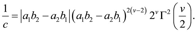
for  where the constant
 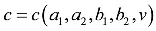 is given by
The density (1.1) is introduced by [7], by using a characterization of Bessel distribution due to the [8]. Reference [8] showed that if U and V are independent chi-squared random variables with common degrees of freedom v, then the distribution of  subject to
 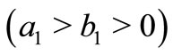 is a Bessel distribution. In a nice generalization, Reference [7] have proved that the joint pdf of
 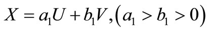 and
and 
 is given by (1.1). They have called this distribution as bivariate Bessel distribution of type I. For more information about Bessel distribution, see [7,8]. It is well-known that under certain condition, the inverse of Fisher Information Matrix (FIM) is the covariance matrix of the estimate of the parameters. The FIM has many application in statistics and other sciences. For an excellent recent references on applications of the FIM see [9]. The aim of this paper is to compute FIM for the bivariate density function (1.1) and is organized as follow: an explicit expression for the FIM for Bivariate Bessel distribution of type I is given in Section 2. Computing FIM for a special case of bivariate density function is given in Section 3. In Section 4, we provide some tools for the numerical computation of the FIM. Some tables of the FIM are also given.
2. An Explicit Expression for the FIM
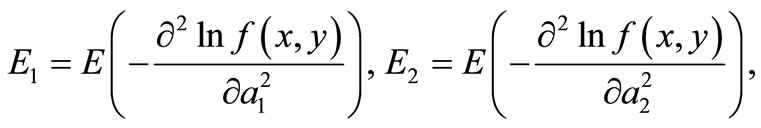
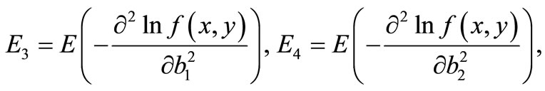
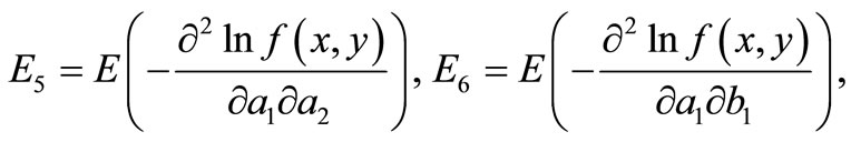
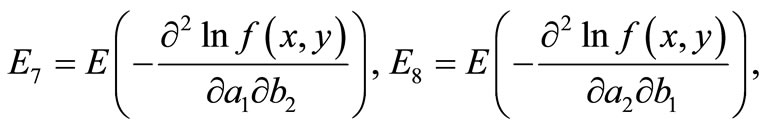
For a given observation  the FIM has the form
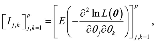 (2.1)
(2.1)
where  and
and  are the parameters of the density. According to (1.1), the unknown vector of parameters is
  The log likelihood of (1.1) for observation
  is Finally,
 (2.2)
(2.2)
Take  and
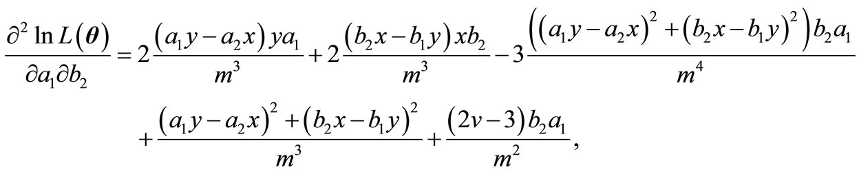
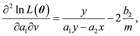
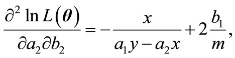
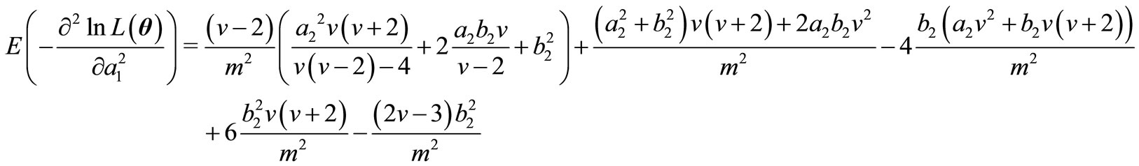
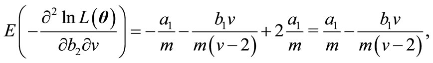
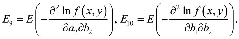
and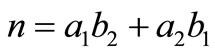 . In the following, we compute all the second derivatives of log likelihood (2.2) subject to parameters.


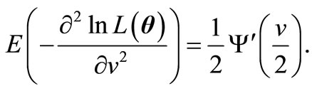
 ,
,
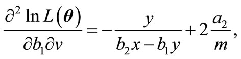

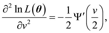
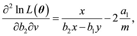
where  is the derivative of digamma function.
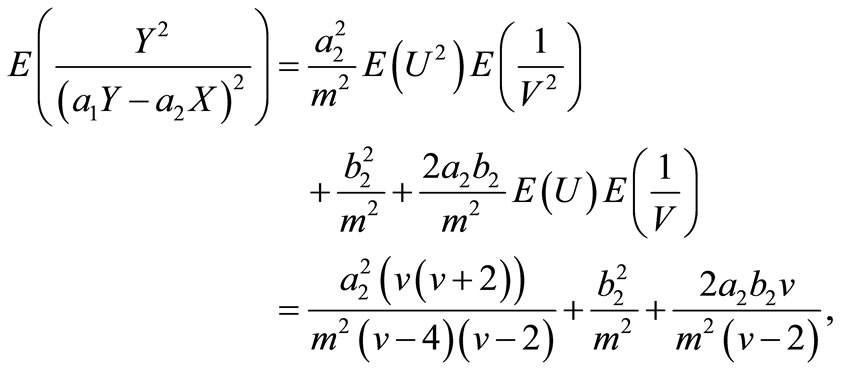
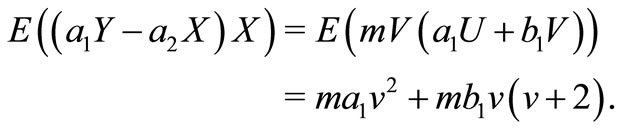
For computing the elements of FIM, following [7], let 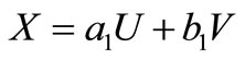 and
and 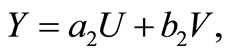 then,
then, 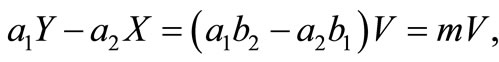 and
and 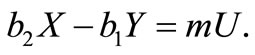
We have found these identities take the computations easy.
At first note that if U has chi-squred distribution with 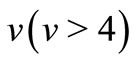 degree of freedom then,
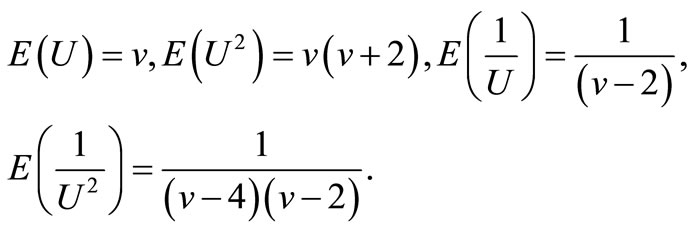
Similarly, we have

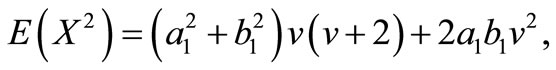
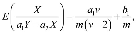

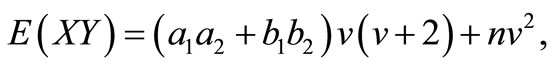
and
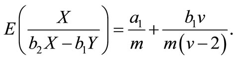
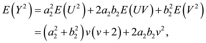
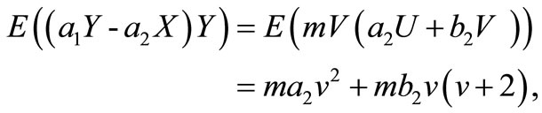
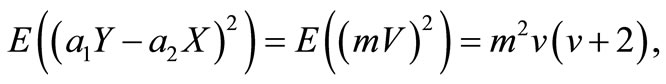
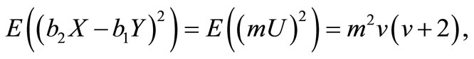
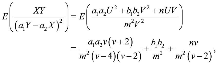
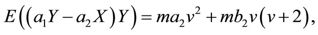
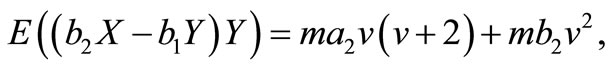
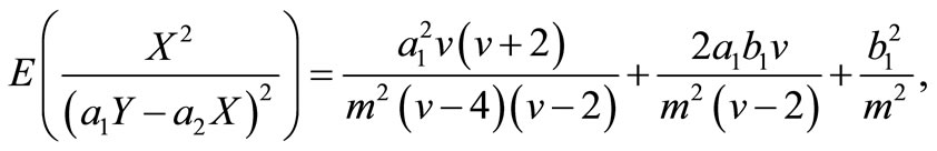
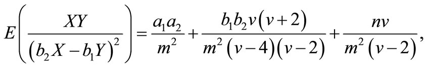
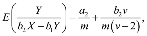
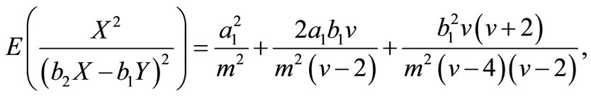
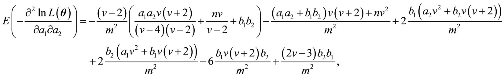
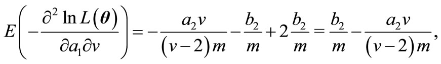
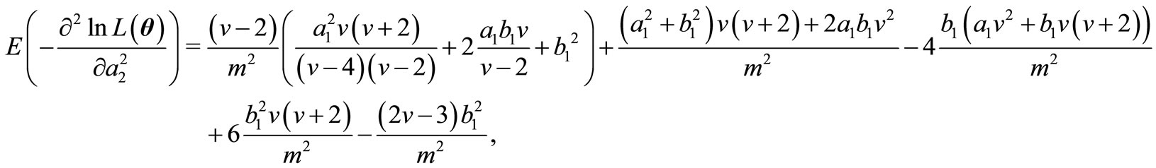
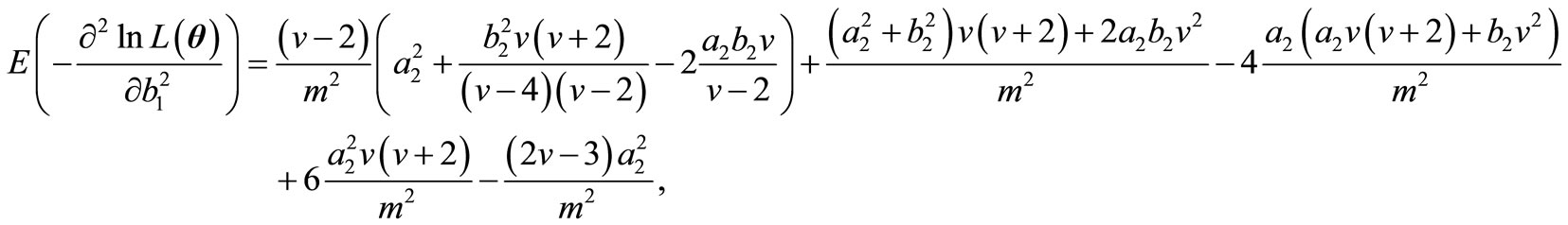
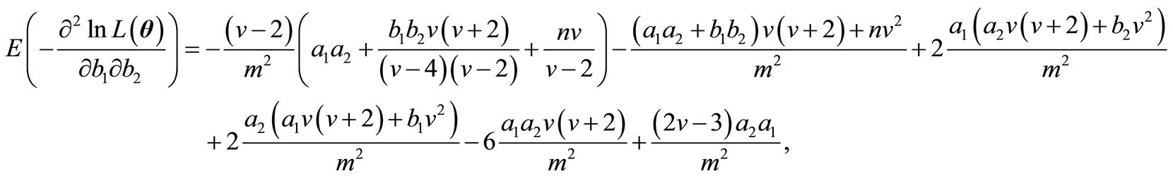
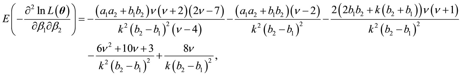
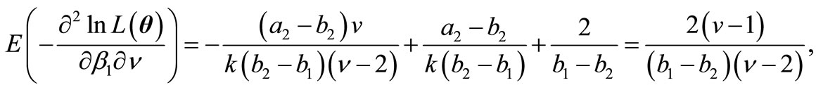
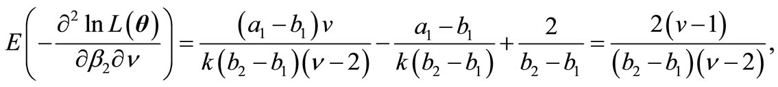
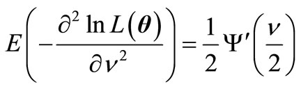
Therefore, the elements of FIM can be calculated as below.


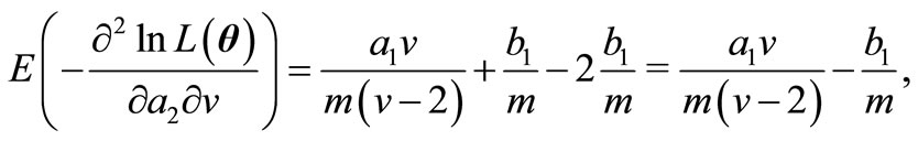
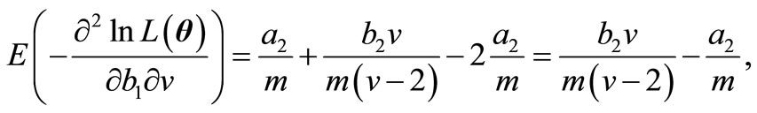
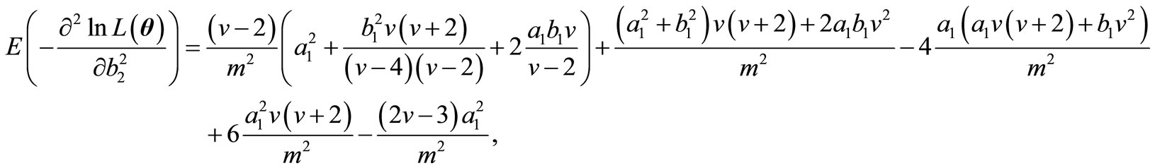
and finally
3. Special Case
Since above experessions are very tedios, we also compute FIM for some assumtions as below. We assume that, 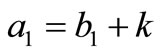 and
and 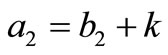 for some fixed k. Then the elements of FIM can be computed as below. As we see the experessions are easier than the former experessoins and the dimension of the parameters is shorter than the peremier parameters.


and finally,
4. Numerical Computation and Tables of the FIM
In this section, some numerical tabulations of the FIM are given to illustrate the computations in the last section.
Take,
and
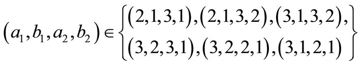
In the Tables 1-6, we have computed the elements of FIM for the Bivariate Bessel distribution of type I, for
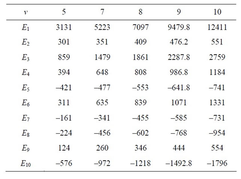
Table 1. Elements of the FIM for (a1, b1, a2, b2) = (2, 1, 3, 1).
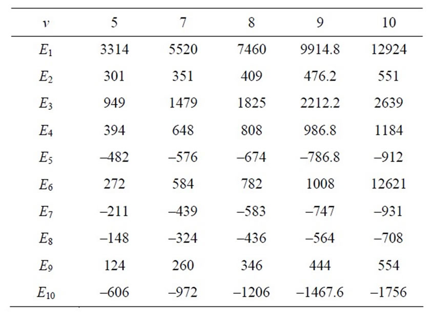
Table 2. Elements of the FIM for (a1, b1, a2, b2) = (2, 1, 3, 2).
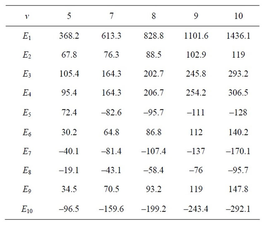
Table 3. Elements of the FIM for (a1, b1, a2, b2) = (3, 1, 3, 2).
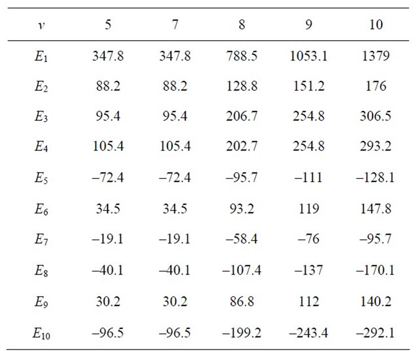
Table 4. Elements of the FIM for (a1, b1, a2, b2) = (3, 2, 3, 1).
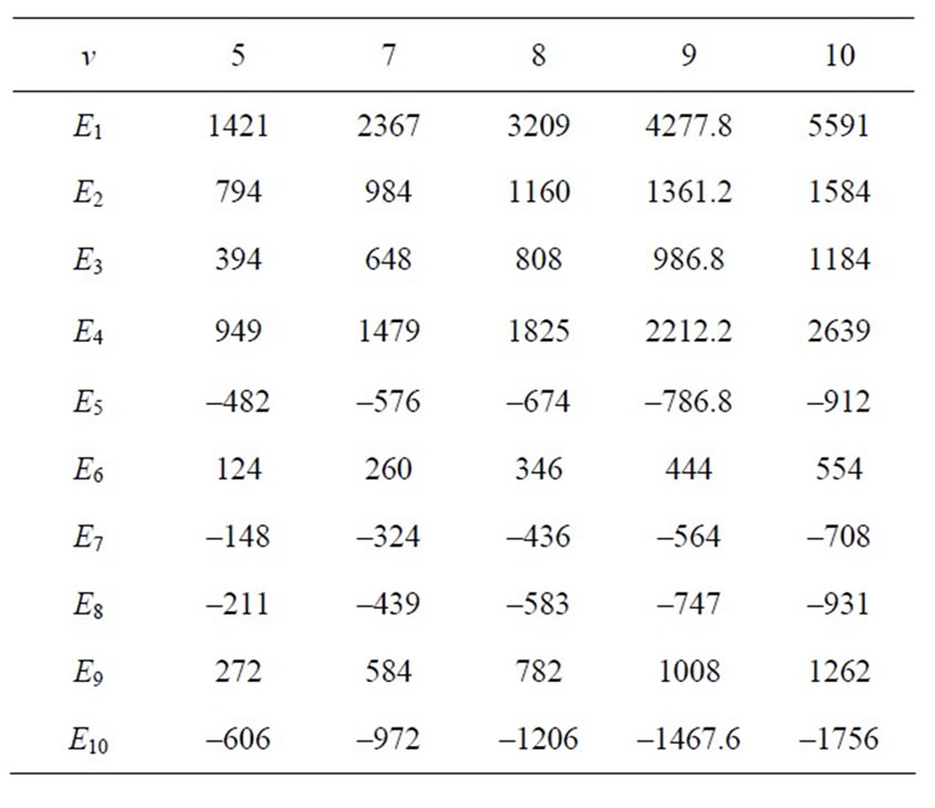
Table 5. Elements of the FIM for (a1, b1, a2, b2) = (3, 2, 2, 1).
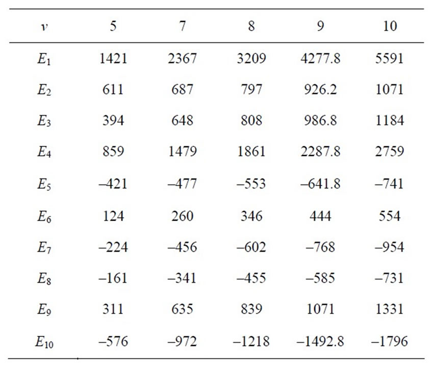
Table 6. Elements of the FIM for (a1, b1, a2, b2) = (3, 1, 2, 1).
different values of
and 
5. Acknowledgements
The authors would like to thank respectful editor in chief and a referee for their helpful comments.
REFERENCES
- A. T. McKay, “A Bessel Function Distribution,” Biometrika, Vol. 24, No. 1-2, 1932, pp. 39-44. doi:10.1093/biomet/24.1-2.39
- R. G. Laha, “On Some Properties of the Bessel Function Distributions,” Bulletin of the Calcutta Mathematical Society, Vol. 46, 1954, pp. 59-72.
- D. L. McLeish, “A Robust Alternative to the Normal Distribution,” Canadian Journal of Statistics, Vol. 10, No. 2, 1982, pp. 89-102. doi:10.2307/3314901
- F. McNolty, “Applications of Bessel Function Distributions,” Sankhya B, Vol. 29, 1967, pp. 235-248.
- L. Yuan and J. D. Kalbfleisch, “On the Bessel Distribution and Related Problems,” Annals of the Institute of Statistical Mathematics, Vol. 52, No. 3, 2000, pp. 438-447. doi:10.1023/A:1004152916478
- L. Devrore, “Non-Uniform Random Variate Generation,” Springer, New York, 1986.
- S. Nadarajah and S. Kotz, “Some Bivariate Bessel Distributions,” Applied Mathematics and Computation, Vol. 187, No. 1, 2007, pp. 332-339. doi:10.1016/j.amc.2006.08.130
- B. C. Bhattacharyya, “The Use of Mackay’s Bessel Function Curves for Graduating Frequency Distributions,” Sankhya, Vol. 6, 1942, pp. 175-182.
- S. Nadarajah, “FIM for Arnold and Strauss’s Bivariate Gamma Distribution,” Computational Statistics and Data Analysis, Vol. 51, No. 3, 2006, pp. 1584-1590. doi:10.1016/j.csda.2006.05.009