Atmospheric and Climate Sciences
Vol.4 No.1(2014), Article ID:42024,22 pages DOI:10.4236/acs.2014.41013
Wind Power Potential in Interior Alaska from a Micrometeorological Perspective
1Department of Mechanical Engineering, Tennessee Tech University, Cookeville, USA
2Department of Atmospheric Sciences, College of Geosciences, Texas A&M University, College Station, USA
3College of Arts and Sciences, University of Washington, Seattle, USA
4Fu Foundation School of Engineering and Applied Science, Columbia University, New York, USA
5Geophysical Institute, University of Alaska Fairbanks, Fairbanks, USA
6Arbeitgruppe Atmosphärische Prozesse (AGAP), Munich, Germany
7Department of Atmospheric Sciences, College of Natural Science and Mathematics, University of Alaska Fairbanks, Fairbanks, USA
Email: *kramm@gi.alaska.edu
Received November 26, 2013; revised December 22, 2013; accepted December 29, 2013
ABSTRACT
The wind power potential in Interior Alaska is evaluated from a micrometeorological perspective. Based on the local balance equation of momentum and the equation of continuity we derive the local balance equation of kinetic energy for macroscopic and turbulent systems, and in a further step, Bernoulli’s equation and integral equations that customarily serve as the key equations in momentum theory and blade-element analysis, where the Lanchester-Betz-Joukowsky limit, Glauert’s optimum actuator disk, and the results of the blade-element analysis by Okulov and Sørensen are exemplarily illustrated. The wind power potential at three different sites in Interior Alaska (Delta Junction, Eva Creek, and Poker Flat) is assessed by considering the results of wind field predictions for the winter period from October 1, 2008, to April 1, 2009 provided by the Weather Research and Forecasting (WRF) model to avoid time-consuming and expensive tall-tower observations in Interior Alaska which is characterized by a relatively low degree of infrastructure outside of the city of Fairbanks. To predict the average power output we use the Weibull distributions derived from the predicted wind fields for these three different sites and the power curves of five different propeller-type wind turbines with rated powers ranging from 2 MW to 2.5 MW. These power curves are represented by general logistic functions. The predicted power capacity for the Eva Creek site is compared with that of the Eva Creek wind farm established in 2012. The results of our predictions for the winter period 2008/2009 are nearly 20 percent lower than those of the Eva Creek wind farm for the period from January to September 2013.
Keywords:Wind Power; Power Efficiency; Wind Power Potential; Wind Power Prediction; WRF/Chem; Micrometeorology; Momentum Theory; Blade Element Analysis; Betz Limit; Glauert’s Optimum Rotor; Balance Equation for Momentum; Equation of Continuity; Balance Equation for Kinetic Energy; Reynolds’ Average; Hesselberg’s Average; Bernoulli’s Equation; Integral Equations; Weibull Distribution; General Logistic Function; Eva Creek Wind Farm
1. Introduction
Countries around the world are becoming more industrialized raising global energy demand. Increased demand has caused problems to arise owing to the consumption of so-called fossil fuels to supply the energy required. This reason has prompted, for instance, the United States to vow that it will reduce its fossil fuel usage. One approach the United States is considering is to supply “20% of the country’s power consumption by wind energy” (US Department of Energy, 2008). The attempt to hinder the so-called anthropogenic global warming by reducing the emission of carbon dioxide (CO2) released by combustion of fossil fuel in electricity generation may also play a role in global energy strategies.
A local reason to consider the potential of wind power is related to an air quality issue. Fairbanks, the only city in Interior Alaska, is facing the challenge to improve its air quality. Since 2006, the city of Fairbanks has been in violation of the 24-hour National Ambient Air Quality Standard (NAAQS). Concentrations of particulate matter of less than or equal to 2.5 μm in diameter (PM2.5) are of concern for air-quality regulations since PM2.5 can affect human health (e.g., [1-4]). Adverse health effects of PM2.5 can be associated with both long-term and short-term exposure (e.g., [5-7]). To decrease health risks, in the United States of America, the 24-h NAAQS for PM2.5 was tightened to 35 μg∙m−3 in 2006. Communities, for which the last three years of PM2.5-monitoring prior to 2006 showed violation of this new standard, were assigned PM2.5-nonattainment areas. These communities have to develop strategies to get into and remain in compliance [8].
In Fairbanks, PM2.5 concentrations have exceeded frequently the new NAAQS in all winters (November to February) since the onset of monitoring in 1999 (see Figure 1). It is not the first time that Fairbanks is affected by an air quality issue. A decade ago or so, the city of Fairbanks was already faced with another air quality issue caused by high levels of carbon monoxide (CO). In its 2002-interim report the Committee on Carbon Monoxide Episodes in Meteorological and Topographical Problem Areas, National Academy of Sciences stated [9]:
“Fairbanks is an extreme example of the roles that meteorology and land topography play in producing air quality problems. In winter, Fairbanks is subject to extreme atmosphere inversions, at times recording inversion strengths of as much as 30˚C (86˚F) per 100 m of altitude. In addition, Fairbanks is situated in a three-sided bowl, surrounded by the Yukon-Tanana uplands; the bowl opens to the Tanana River Flats toward the south and southeast. Although Fairbanks is not heavily populated
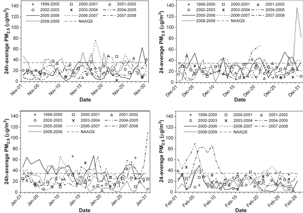
Figure 1. Temporal evolution of 24-h average PM2.5 concentrations for 1999 to 2009 for (upper left to lower right) November, December, January, and February (adopted from Tran and Mölders [8]).
and has no major air-pollution-producing industries, its meteorological and topographical characteristics make the city susceptible to high ambient CO concentrations in winter. The atmospheric inversions and low wind speeds that commonly occur during winter are extremely effective in trapping the products of incomplete combustion, including CO, that are emitted at ground level”.
Mölders and Kramm [10] described the situation in a more detailed manner. They stated:
“The radiation flux balance is mainly negative and leads to the formation of near-surface inversions. In addition, calm winds accompanied by less shear production of turbulent kinetic energy (TKE) often prevail over Interior Alaska. Under such weather conditions, the stratification of the atmospheric layers in the vicinity of the earth’s surface becomes extremely stable. Such weather situations typically lead to huge air quality problems. Air layers close to the ground are strongly polluted by gaseous and particulate matter (PM) released by the combustion of huge amounts of fossil fuel for heating and electricity production and of gasoline in the engines of cars required to save life under extremely low air temperatures. Long-lasting inversions cap these air layers and strongly hinder the export of polluted air into unpolluted air layers aloft especially during the occurrence of calm winds. The emitted PM and gaseous compounds like carbon monoxide, sulfur dioxide, and nitrogen oxides accumulate under such extremely stable conditions and lead to frequent violations of Environmental Protection Agency (EPA) regulations in Fairbanks, the only city in Interior Alaska”.
Several solutions are being considered to reduce anthropogenic emission of gaseous and particulate matter. Since the production of electricity contributes to this emission, one solution under consideration may be the installation of wind farms at one or more locations in Interior Alaska. Unfortunately, as reported by Wendler and Shulski [11], the wind speed in the Fairbanks area is very low (see Figure 2). Thus, Fairbanks has to be excluded as an appropriate site for the generation of electricity by the conversion of kinetic energy transported by the wind because the mean daily wind speed is lower than the cut-in wind speed of most wind turbines suitable for wind farms. The same is true for most locations in Alaska for which reliable meteorological records are available. Cooney and Kramm [12] analyzed the daily wind data from twenty first-order weather stations (see Table 1) for the winter period October 1, 2008 to April 1, 2009 (denoted hereafter as winter period 2008/2009) to determine which locations received sufficient wind power to support a wind farm. Their results indicate that only four locations, namely St. Paul Island, Cold Bay, Bethel, and Kotzebue, would be very good candidates for wind farms. However, when determining the best location for a wind farm, one must assess not only the wind power potential, but also endangered species, avian migrations/habitats, and if there are wetlands/protected areas around the location. St. Paul Island, located in the Bering Sea, for instance, is home to millions of seabirds nesting in colonies along its steep shores. Rare birds are found here each year during spring migration. Also, St. Paul Island is considered a top North American bird watching destination [12].
Since 2003, the local energy producer, Golden Valley Electric Association (GVEA), has been researching the possibility of constructing a wind power facility at Eva Creek located approximately 23 km northeast of Healy (63.97˚N, 149.13˚W), Alaska at the top of the Ferry mining road. None of the twenty first-order stations listed in Table 1 is close to this location. However, GVEA reported on its website
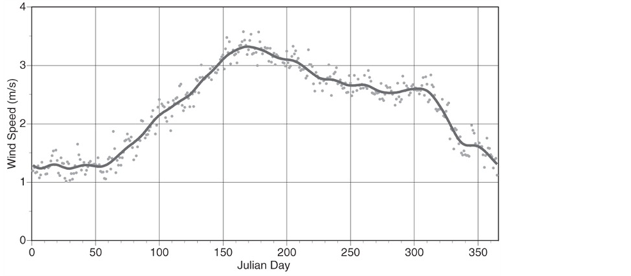
Figure 2. Mean annual course of the mean daily wind-speed values for Fairbanks, 1946-2006. The solid line represents the 11-point smoothed values (adopted from Wendler and Shulski [11]).

Table 1. List of twenty fist-order stations for organization into station numbers (adopted from Cooney and Kramm [12]).
(http://www.gvea.com/energy/evacreek) that it had installed its first meteorological wind monitoring towers in 2003 and for further testing two 80-meter meteorological towers at the Eva Creek site and one 50-meter meteorological tower on Walker Dome in October 2009. Figure 3 shows wind data for September 2007. It illustrates a high variability of wind speed during that period, where often the mean wind speed drops below the cut-in wind speed of a typical wind turbine for many hours. According to Newton and Wyman [13], these wind data would result in an average recorded available power of 8.54 MW. Since the rated power is 24.6 MW, the average capacity factor would be 34.7 percent, i.e., slightly higher than that realized by the Eva Creek wind farm (see Figure 4) in September 2013.
In June 2011, the Eva Creek Wind Farm project obtained final approval. Construction at the site began early in 2012. The commercial operation has started in October 2012 (see the GVEA website). In addition, to mitigate PM2.5 levels, wind farms like the Eva Creek wind farm reduce Alaska’s oil consumption and bring the GVEA one step closer to fulfilling its Renewable Energy Pledge. The pledge was adopted in 2005 and calls for 20 percent of the system’s peak load to come from renewable sources by 2014 (see the GVEA website).
The first-order weather station Big Delta is located at the confluence of the Tanana River and the Delta River approximately 14 km north-northeast of the city of Delta Junction. Delta Junction was proposed by Alaska Environmental Power (AEP) contracted with Electrical Power Systems Inc. (EPS), an independent electricity producer, as an alternative location (or even an additional one) for
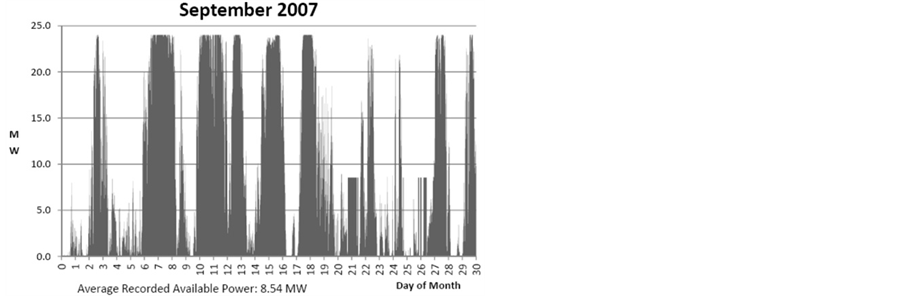

Figure 4. The Eva Creek wind farm (adopted from Golden Valley Electric Association).
a wind farm. Here, a small scale wind farm located approximately 7 km east of Delta Junction is currently operating.
Wind power might also be helpful to reduce the costs in running the Poker Flat Research Range, the world’s only scientific rocket launching facility owned by a university. Poker Flat is located approximately 48 km north of Fairbanks and is operated by the University of Alaska’s Geophysical Institute. Therefore, Poker Flat was also considered in our study.
In 2011, an independent assessment of the Eva Creek Wind Farm project was already performed by Hinzman and Kramm [14]. They used the wind field predictions (hourly basis) for the winter period 2008/2009 (performed by Mölders using the Alaska-adapted WRF/Chem setup, see Section 3) and the power curve of the propeller-type turbine REpower MM92 (cold climate version, CCV) matched by the sigmoidal function
 (1.1)
(1.1)
where v is the wind speed (expressed in m∙s−1), and A = 2053.8 kW, B = 14.5 kW, k = 0.1139 s∙m−1, and d = 4.705 are constants. Their results are illustrated in Figure 5. Based on their findings, Hinzman and Kramm [14] suggested that the Eva Creek wind farm might serve to deliver cheap energy for Alaskans even though the average power output would only be a quarter of the rated power. The current study expands on their research by considering three different sites in Interior Alaska, namely Eva Creek, Delta Junction, and Poker Flat, in estimating the average power that can be generated at each site, where power characteristics of five different wind turbines were alternatively considered.
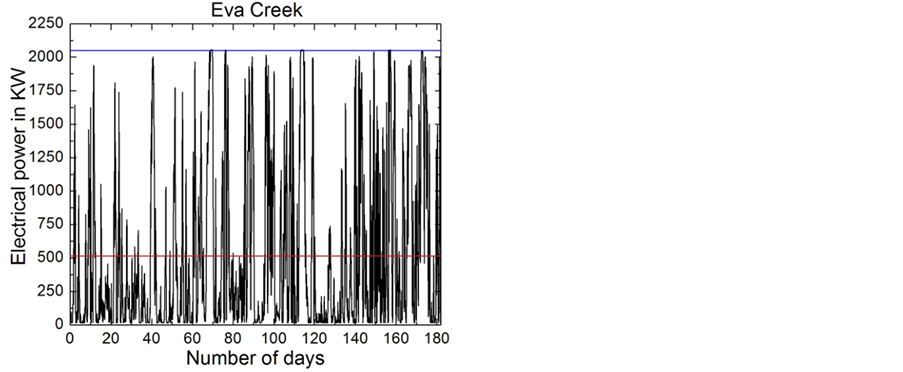
Figure 5. Wind power output of the propeller-type wind turbine REpower MM92 (CCV) predicted for the Eva Creek site with respect to the winter period 2008/2009. The blue line shows the rated power and the red line the mean power (adopted from Hinzman and Kramm [14]).
A wind turbine acts as a sink of kinetic energy transported by the wind field (divergence effect). This effect was not considered when the wind fields were predicted. As shown in Figure 4, the Eva Creek wind farm consists of sparsely distributed turbines. In such a case the aerodynamic effect caused by the wind turbines might be negligible. However, in case of larger wind farms it may become important. Thus, there is an urgent need to parameterize this aerodynamic effect in mesoscale numerical models of the atmosphere if they are to be considered to predict the electricity generated by larger wind farms.
To assess the wind power potential over an area like Interior Alaska the use of a numerical weather prediction (NWP) model is indispensable in avoiding time-consuming and expensive tall-tower observations at various locations in an area that is characterized by a relatively low degree of infrastructure outside of Fairbanks. Storm et al. [15] for West Texas and southern Kansas and Storm and Basu [16] for the United States Great Plains assessed the feasibility of the Weather Research and Forecasting (WRF) model [17] to predict Low-Level Jets (LLJs) and low-level wind shear characteristics. Storm et al. [15] found that WRF can capture some of the essential characteristics of observed LLJs, and offers the prospect of improving the accuracy of wind resource estimates and short-term wind energy forecasts. The results of Storm and Basu [16] indicate that WRF qualitatively captures several low-level wind shear characteristics. However, they pointed out that room for physics parameterization improvements to reliably represent the lower part of the atmospheric boundary layer (ABL) definitely exists.
Mölders and collaborators [10,18] already assessed the performance of WRF and WRF/Chem to simulate the ABL characteristics over a sub-Arctic area during different winter periods. Mölders and Kramm [10] tested various WRF configurations for an extremely cold five day weather period (January 27, 2008 to February 2, 2008) with multi-day inversions over Interior Alaska. Comparison of the simulations with data of surface observations at 45 sites and radiosondes launched at Fairbanks and McGrath every 12 hours showed that WRF’s performance for these inversions strongly depends on the physical packages chosen. Simulated near-surface air temperatures as well as dew-point temperatures differ about 4 K on average depending on the physical packages used. All WRF simulations underlined the difficulties in capturing the full strength of the near-surface temperature inversion and in simulating strong variations of dew-point temperature profiles. The greatest discrepancies between simulated and observed vertical profiles of temperature and dew-point temperature occur around the levels of great wind shear. Out of the configurations tested the radiation schemes of the Community Atmosphere Model combined with the Rapid Update Cycle land surface model and modified versions of the Medium Range Forecast model’s surface layer and ABL schemes capture the inversion situation best most of the time.
Mölders et al. [18] used data from a Doppler SOund Detection And Ranging (SODAR) device, twice-daily radiosondes, 33 surface meteorological and four aerosol sites to assess the ability of WRF inline coupled with a chemistry package (WRF/Chem) to capture ABL characteristics in Interior Alaska during low solar irradiation (November 1, 2005 to February 28, 2006). Biases determined based on all available data from the 33 sites over the entire episode are 1.6 K, 1.8 K, 1.85 m∙s−1, −5˚, and 1.2 hPa for temperature, dewpoint temperature, wind speed, wind direction, and sea-level pressure, respectively. The SODAR-data reveal that WRF/Chem over/under-estimates wind speed in the lower (upper) ABL. WRF/Chem captures the frequency of LLJs, but overestimates the strength of moderate LLJs. Data from the four aerosol sites suggest large underestimation of PM10, and NO3 at the remote sites and PM2.5 at the polluted site. Difficulty in capturing the temporal evolution of aerosol concentrations coincides with difficulty in capturing sudden temperature changes, underestimation of inversion-strengths and timing of frontal passages.
In the following, a description of the theoretical background of wind power prediction from a micrometeorological perspective is presented (Section 2). Based on the local balance equation of momentum and the equation of continuity we derive the local balance equation of kinetic energy for macroscopic and turbulent systems, and in a further step, Bernoulli’s equation and integral equations that customarily serve as the key equations in momentum theory and blade-element analysis. It mainly follows that of Kramm et al. [19] and serves to understand the generation of electricity by extracting kinetic energy from the wind field by using a propeller-type wind turbine and its inherent limitation characterized by power efficiency. In accord with Storm et al. [15], Storm and Basu [16], Mölders and Kramm [10], Mölders et al. [18], and Hinzman and Kramm [14], we also consider low-level wind field characteristics predicted by WRF/Chem [20] to assess the wind power potential over Interior Alaska. A brief model description of WRF and the evaluation of the predicted wind fields are given in Section 3. The methods of data analysis are described in Section 4. The results of wind power prediction for three different locations by considering five different propellertype wind turbines are presented and discussed in Section 5.
2. Micrometeorological Background
2.1. The Governing Equations for the Macroscopic System
To outline the generation of electricity by extracting kinetic energy from the wind field we have to consider the local balance equations for momentum (i.e., Newton 2nd axiom), Equation (2.1), and total mass, Equation (2.2), for a macroscopic system given by [21,22]
 (2.1)
(2.1)
and
 (2.2)
(2.2)
Here, ρ is the air density, t is time, v is the velocity of the flow, J is the Stokes stress tensor, E is the identity tensor, p is the air pressure, φ is the gravity potential, and Ω is the angular velocity of the Earth. Both J and E are symmetric second-rank tensors. The 1st term of the left-hand side of Equation (2.1) describes the local temporal change of momentum, and the 2nd term represents the exchange of momentum between the system under study and its surroundings, where  exerts on the boundary of this system. The 1st term on the right-hand side of Equation (2.1) represents the gravity force, and the 2nd one the Coriolis force. Equation (2.2) is called the equation of continuity. The local balance equations various energy forms (i.e., internal energy, kinetic energy, potential energy, and total energy), various water phases (i.e., water vapor, liquid water, and ice), and atmospheric trace constituents can be derived from integral balance equations (e.g., [21,22]).
To deduce the local balance equation for the kinetic energy of the flow, Equation (2.1) has to be scalarly multiplied by the velocity vector v. In doing so, yields
 (2.3)
(2.3)
where the identities

and  have been used. Note that the colon expresses the so-called double-scalar product of the tensor algebra. Furthermore,
 . The 1st term of the left-hand-side of Equation (2.3) describes the local temporal change of kinetic energy, and the 2nd term the energy exchange of the system with its surroundings which is performed by the surrounding air on the boundary of the system. The 1st term of the right-hand-side represents the conversion of potential energy into kinetic energy or vice versa, the 2nd term describes the reversible work rate of expansion
  or contraction
 , and the 3rd term represents the irreversible work rate owing to viscous friction. This term describes the dissipation of kinetic energy into the reservoir of heat. The term of our primary interest reads
 (2.4)
(2.4)
It describes the transport of kinetic energy by the flow, and may be called the kinetic energy stream density or the wind power density.
2.2. The Governing Equations for the Turbulent System
The ABL is mainly governed by turbulent motion. Consequently, the use of the macroscopic balance Equations (2.1) to (2.3) is rather impracticable. Therefore, these balance equations are commonly averaged in the sense of Reynolds [23]. However, conventional Reynolds averaging will lead to various short-comings in the set of governing equations for the turbulent atmospheric flow, even if the averaging techniques can accurately be performed [24]. If we ignore, for instance, density fluctuation terms, the possibility to describe physical processes as a whole will clearly be restricted (see also [25,26]). The key questions are (1) how to average the governing macroscopic equations in the case of turbulent atmospheric flows, and (2) what are the consequences of such an averaging for momentum and total mass as well as various energy forms.
As demonstrated by Pichler [27], Cox [28], Kramm et al. [29], Thomson [30], Venkatram [31], Kramm and Meixner [24], and Kowalski [32], the density-weighted averaging procedure suggested by Hesselberg [33],
 , (2.5)
is suitable to formulate the local balance equations for turbulent systems. Here,  is a field quantity like the wind vector, v, the specific internal energy, e, and the specific enthalpy, h. The overbar
  characterizes the conventional Reynolds [23] mean. Whereas the hat
  denotes the density-weighted average according to Hesselberg [33] and the double prime (") marks the departure from that. It is obvious that
 . The Hesselberg mean of the wind vector, for instance, is given by
 . Note that intensive quantities like pressure p and air density ρ are only averaged in the sense of Reynolds (for arithmetic rules, see [27,29,34-36]).
Hesselberg’s averaging calculus leads to several prominent advantages (e.g., [27-29,33,34]): (1) The equation of continuity,
 , (2.6)
keeps its form, and (2) the mean value of kinetic energy can exactly be split into the kinetic energy of the mean motion and mean value of the kinetic energy of the eddying motion, i.e.,
 . (2.7)
This fact is especially important in the theoretical description of the extraction of the kinetic energy from the wind field for generating electricity. As pointed out by Thomson [30], the use of density-weighted averages is the common way to define averages in studies of highly compressible turbulent flows (see [24,37]), probably the most natural way to define averages. The kinetic energy of the mean motion is usually abbreviated by MKE, and the kinetic energy of the eddying motion is usually called the turbulent kinetic energy abbreviated by TKE.
Hesselberg’s average procedure will generally be applied in this study. The Hesselberg average can be related to that of Reynolds by (e.g., [24,28,29,35,38])
 , (2.8)
where the prime denotes the deviation from the Reynolds mean. Obviously, the different averages,  and
and , are nearly equal if
  as used, for instance in case of the Boussinesq approximation. In case of a nearly incompressible fluid the distinction between
  and
and  is not needed because the condition
  is clearly fulfilled. However, to avoid confusion, we do not change our notation.
In the averaged form, the local balance equation for momentum for the turbulent atmosphere reads (e.g., [24, 27,33-36,39]):
 (2.9)
(2.9)
where  is the Reynolds stress tensor. It results from averaging the term
  in Equation (2.1) leading to
 .
.
Similar local balance equations can be derived for various energy forms (i.e., internal energy, kinetic energy, potential energy, and total energy), various water phases (i.e., water vapor, liquid water, and ice), and gaseous and particulate atmospheric trace constituents (e.g., [24,27,28, 34,36,39,40]). State-of-the-art numerical models like WRF are based on these local balance equations for the turbulent atmosphere.
Averaging Equation (2.3) provides the local balance equation for the kinetic energy
 (2.10)
for turbulent systems. Obviously, the local derivative with respect to time contains the MKE and the TKE as outlined by Equation (2.7). Assuming, for instance, steady-state condition leads to

This means that under this condition the total kinetic energy is time-invariant, but MKE can be converted into TKE.
In the inertial range, the TKE is transferred from lower to higher wave numbers until the far-dissipation range is achieved. Here, the conversion of kinetic energy into heat energy by direct dissipation  and turbulent dissipation
  occurs. Despites the fluctuations of the wind vector are usually small as compared to the mean wind vector
  the opposite is true for the gradients of these quantities
 . This phenomenon is connected with a great intensity of rotation and is characteristic for all turbulent flows. Except for the immediate vicinity of solid walls, a consequence is that turbulent dissipation exceeds that of direct dissipation by several orders of magnitude depending on the Reynolds number (e.g., [41]). Furthermore, the mean kinetic energy stream density reads
 . (2.11)
This equation describes the transfer of MKE and TKE by the mean wind field as well as the transfer of turbulent kinetic energy by the eddying wind field. Neglecting the turbulent effects leads to the mean kinetic energy stream density
 . (2.12)
This simplified version of the mean kinetic energy stream density plays the key role in wind power studies. The magnitude of this stream density is given by
 . (2.13)
where . This quantity expresses that the wind power density is proportional to the cube of the wind speed. Furthermore, the rotor of a wind turbine causes a divergence effect, i.e.,
 .
.
The local balance equation of MKE can be derived by scalarly multiplying Equation (2.9) by . One obtains
 (2.14)
Subtracting this equation from Equation (2.10) yields
 (2.15)
or
 (2.16)
where
 (2.17)
is a non-dimensional parameter that serves to characterize the thermal stability of the turbulent flow. This stability parameter expresses the relative importance of the two TKE-terms. It may be interpreted as a generalized Richardson number. The difference between the wellknown flux-Richardson number and the generalized Richardson number introduced here results from the parameterisation of  (e.g., [24]). Besides the vertical effects, also horizontal effects have to be considered under certain circumstances. In case of
 , mechanically produced TKE is mainly consumed by Archimedean effects. Consequently, there exists a critical
  -value given by
 . It characterizes the fact that the mechanical gain of TKE is equal to the thermal loss of TKE, i.e., the term
  becomes equal to zero, and the net production rate of TKE vanishes. As the turbulent dissipation still acts as a sink of TKE, the turbulent flow becomes more and more viscous (laminar). In case of
 , TKE is generated mechanically and thermally. When the mechanically generated TKE is much smaller than the thermal gain of TKE, and, hence, negligible, free convective conditions
  occur. In the remaining range, mixed convective conditions prevail
 . Note that Equation (2.15) is a 2nd-order balance equation. It is the only balance equation that additionally arises from averaging a macroscopic balance equation (e.g., [24, 36,39]). Furthermore, in meteorological models of the mesoscale like WRF the balance equation of TKE (2.15) is used to derive the eddy diffusivities for momentum and via the turbulent Prandtl number and the speciesdependent turbulent Schmidt numbers—the eddy diffusivities for sensible heat, and water vapor. This method of parameterization is known as one-and-a-half-order closure (e.g., [24]).
From the perspective of the generation of electricity by extracting kinetic energy from the wind field Equations (2.6), (2.9), and (2.14) play a key role. To obtain a tractable set of equations, effects caused by molecular and turbulent friction, i.e.,  ,
,  , and
, and  , are usually ignored. In addition, the conditions of steady-state,
  , and local incompressibility,
  , are presupposed. Thus, the set of approximated equations reads
 , (2.18)
 , (2.19)
and
 . (2.20)
2.3. The Bernoulli Equation
By assuming local incompressibility,  , Equation (2.20) becomes
 . (2.21)
Based on this condition, Bernoulli’s equation which plays an important role in describing the conversion of wind energy can simply be derived by considering this condition along a streamline. In accord with the natural coordinate frame for streamlines, the Nabla operator reads
 . (2.22)
The unit vectors ,
,  , and
, and  form a right-handed rectangular coordinate system (trihedron) at any given point of a curve in space like a streamline or a trajectory. Here, the subscript s characterizes the streamline-related quantities. The velocity vector at a given point along the streamline is given by
 , where
  is its magnitude,
  is the unit tangent of the streamline, and
  is the unit tangent of the corresponding trajectory. The unit vectors
  and
and  are called the principal normal and the binormal, respectively (e.g., [42]).
In accord with Equation (2.22), the condition (2.21) results in
 (2.23)
This means that for any value of  the condition
 (2.24)
must be fulfilled along a streamline. Equation (2.24) is Bernoulli’s equation (e.g., [22,43,44]). Even though air density is considered as spatially constant, Bernoulli’s equation can often be applied to atmospheric flows. If the streamlines are mainly horizontally oriented and the variation of the gravity potential with height is small like in case of the swept area of a wind turbine, the gravity effect may also be considered as constant. Thus, Equation (2.24) results in
 (2.25)
This approximation of Bernoulli’s equation serves, for instance, to derive the Rankine-Froude theorem (see Equation (2.37)).
2.4. The Integral Equations
The integration of Equations (2.18) to (2.20) over a time-independent control volume, Vc, encompassing the rotor of the wind turbine, leads to [19,45]
 , (2.26)
 (2.27)
and
 . (2.28)
In accord with Gauss’ integral theorem, Equation (2.26) and the left-hand side of Equation (2.27) can be written as
 (2.29)
and
 (2.30)
where  is the thrust. Since
  is a second-rank tensor, it is advantageous to scalarly multiply Equation (2.27) by the unit vector
  from the left to get a more tractable equation. In doing so, one obtains:
 (2.31)
Here,  is the axial force acting on the rotor of a propeller-type wind turbine (e.g., [19,45]). If we assume that the axial direction coincides with any horizontal direction, the term
  will be nearly equal to zero. Since the Coriolis acceleration is given by

where  is the latitude, and
 ,
,  , and
, and  are the components of the mean wind vector in west-east direction (characterized by the unit vector
 ), south-north direction (characterized by the unit vector
 ), and the vertical direction (characterized by the unit vector
 ), respectively; the term

is very small for any value smaller than the cut-out wind speed because . Thus, this term can be ignored, and Equation (2.31) may be approximated by
 . (2.32)
The second term of the left-hand side of this equation is usually ignored in the blade element momentum (BEM) theory. However, as pointed out by Goorjian [46] and Sørensen [45], this term is not zero. Since  may be expressed by
 , where
 ,
,  , and
, and  are the cylindrical polar coordinates, respectively; and
 ,
,  , and
, and  are the corresponding unit vectors pointing in axial, radial, and azimuthal direction.
The azimuthal velocity component acting on the rotor at radius  causes a torque given by
 . (2.33)
According to Gauss’ integral theorem, the left-hand side of Equation (2.28) can be written as
 . (2.34)
This term represents the power extracted by the rotor of the wind turbine. In case of a quasi-horizontal flow the right-hand side of Equation (2.28) may be neglected because  is quasi-perpendicular to
 . Note that the effect of the gravity potential was already considered as negligible in case of Bernoulli’s Equation (2.25). Apparently, the integral relation (2.34) underlines the importance of Bernoulli’s equation in wind power studies. As documented by Sørensen [45] and Kramm et al. [19], Equations (2.32) to (2.34) are key equations for momentum theory and blade-element analysis.
2.5. The Power Efficiency
Figure 6 illustrates the so-called Lanchester-Betz-Joukowsky (LBJ) limit (e.g., [45,48,49]) for the maximum of the (wind) power efficiency (e.g., [50]),
 (2.35)
that is based on the axial momentum theory (i.e., onedimensional problem) developed by Rankine [51], W. Froude [52], and R. E. Froude [53]. Here,  , where
  is the wind speed of the undisturbed wind field far upstream of the turbine, and
  is the wind speed of the undisturbed wind field far downstream of the turbine. Furthermore,
  is the power extracted from the wind field by the turbine, and, in accord with Equation (2.13),
 (2.36)
is the power of the undisturbed wind field, where  is an area equivalent to that swept out by the rotor of a propeller-type wind turbine (e.g., [47]). The quantity
  is referred to as the axial interference factor, where
  is the axial velocity in the rotor plane. The factor is a measure of the influence of the wind turbine on the air (e.g., [45,47,49,54,55]). Using the Rankine-Froude theorem (e.g., [50]),
 , (2.37)
yields . Obviously,
  leads to
 , and
, and  to
to . To determine the maximum of power efficiency, the first derivative test,
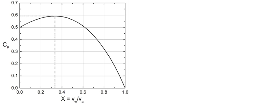
Figure 6. The Lanchester-Betz-Joukowsky limit. The solid line represents Equation (2.35) and the dashed lines characterizes the maximum of the power efficiency.
 , and the second derivative test,
 , have to be used. The first derivative test leads to
 , and the second derivative test provides that for this value of
  the power efficiency reaches its maximum (see Figure 6). Inserting
 into Equation (2.35) yields the LBJ limit (e.g., [45,47,49,50,54,56])
 . (2.38)
Note that  with
with  provides the same result.
The LBJ limit is based on a simplified description of the flow field. Even though the flow field exhibits a pure axial behavior in front of the rotor, by interacting with the rotor also velocity components in radial and azimuthal directions occur in the rotor plane and in the wake. To consider these rotational effects Glauert [57] developed a simple model for the optimum rotor. In his approach, Glauert treated the rotor as a rotating axisymmetric actuator disk, corresponding to a rotor with an infinite number of blades [45,47,49]. Glauert [57] derived the following expression for the power efficiency:
 , (2.39)
where ,
,  is the tip-speed ratio,
  is the azimuthal interference factor, and
  is the angular velocity of the rotor. In case of the optimum rotor the azimuthal interference factor and the axial interference factor are related to each other by
 . (2.40)
This means that the optimum axial interference factor is no longer a constant, but depends on the rotation of the wake, and that the operating range for an optimum rotor is . As illustrated in Figure 7, the maximum of the power efficiency depends on the tip-speed ratio. It approaches the LBJ limit of 16/27 at large tipspeed ratio only [45,47,49].
Based on their theoretical considerations, Okulov and Sørensen [49,55] showed that the power coefficient for a propeller of a finite number of blades approaches that of Glauert’s [57] optimum actuator disk, when the number of blades increases (see Figure 8). They also compared the optimum conditions for finite number of blades as a function of tip-speed ratio for two different models: (a) Joukowsky rotor with constant circulation along the blade,
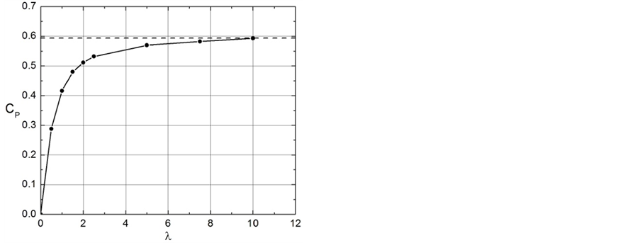
Figure 7. Power coefficient vs. tip-speed ratio for Glauert’s [56] optimum actuator disk. The data are taken from Wilson and Lissaman [47].
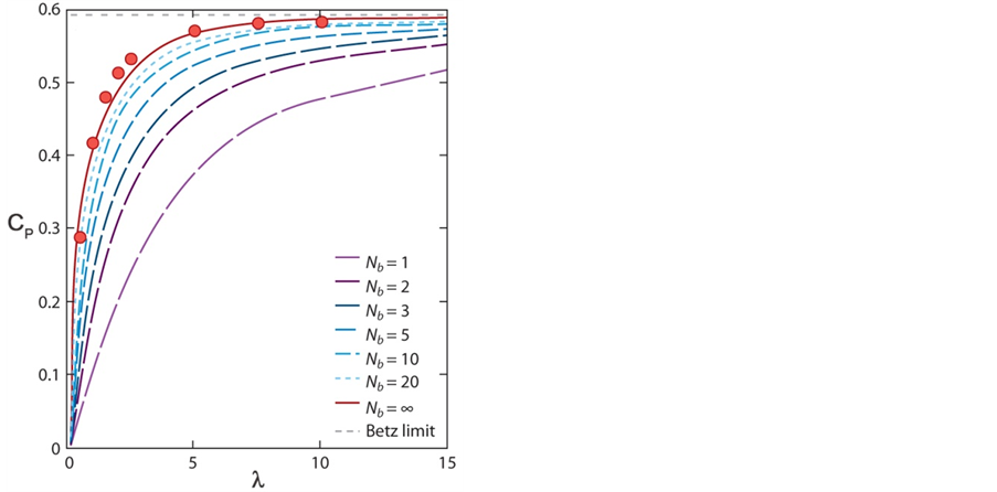
Figure 8. Power coefficient vs. tip-speed ratio for different numbers of blades of an optimum rotor. Points represent the general momentum theory shown in Figure 7 and dashed and solid lines represent the theory of Okulov and Sørensen [49] (adopted from Sørensen [45]).
and (b) Betz rotor with circulation given by Goldstein’s function [55]. They found that for all tip-speed ratios the Joukowsky rotor achieves a higher efficiency than the Betz rotor, but the efficiency of the Betz rotor is larger if we compare it for the same deceleration of the wind speed [55].
Figure 9 illustrates the wind power density for a real propeller-type wind turbine. Also shown are the magnitude of the kinetic energy stream density  given by Equation (2.13), and
  weighted by the LBJ limit. Obviously, for higher wind speeds the difference between the LBJ limited value and the real wind power density becomes larger and larger. This means that the
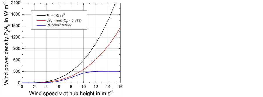
Figure 9. Wind power density  of the wind turbine REpower MM92. Also shown are the wind power density
  given by Equation (2.13), and
  weighted by the LBJ limit.
rotor and blade geometries may be improved to obtain a higher wind power density.
To parameterize in mesoscale numerical models of the atmosphere the behavior of a wind turbine to act as a sink of kinetic energy transported by the wind field (divergence effect), the wind power density related to the power curve (see Figure 9) may be considered.
3. The Prediction of the Wind Field
3.1. Model Set-Up
One of the first steps in assessing the feasibility of a wind energy project is estimating the power that can be generated by a wind turbine at various locations under consideration. This estimation requires knowledge of the local wind field distribution and information on the power output of a turbine at given wind speeds [56].
As mentioned before, for our assessment of the wind power potential at different locations in Interior Alaska we use NWP wind fields for the winter period 2008/2009 provided by the Alaska-adapted WRF/Chem setup (see [18,20]) to avoid time-consuming and expensive talltower observations being carried out at various locations in an area of relatively low degree of infrastructure. The Alaska-adapted WRF/Chem setup includes: 1) the WRFSingle-Moment cloud-microphysics scheme of Hong and Lim [58], 2) the cumulus-ensemble approach of Grell and Dévényi [59], 3) the Goddard two-stream, multi-band model, 4) the Rapid Radiative Transfer Model of Mlawer et al. [60], 5) Janjić’s [61] parameterization schemes for the ABL and the atmospheric surface layer (ASL), 6) the land-surface model of Smirnova et al. [62], 7) the gas-phase chemical mechanism of Stockwell et al. [63], 8) Madronich’s [64] photolysis-rates calculation, 9) Wesely’s [65] deposition module with the modifications introduced by Mölders et al. [20], and 10) the Modal Aerosol Dynamics Model for Europe (MADE; Ackermann et al. [66]) and Secondary Organic Aerosol Model (SORGAM; Schell et al. [67]).
The model domain centered over Fairbanks covered Interior Alaska (Figure 10) with a horizontal grid-increment of 4 km and a vertically stretched grid to 100 hPa.
The initial conditions for the meteorological, snow and soil quantities were interpolated from the 1˚ × 1˚, 6 h-resolution National Centers for Environmental Prediction global final analyses. This dataset also served to downscale and provide downscaled meteorological boundary conditions [20].
WRF/Chem was run in forecast-mode for the entire winter period 2008/2009, where the meteorological fields were initialized every five days (for more details on the model set-up and the initialization of the distributions of the atmospheric trace constituents, see Mölders et al. [20]).
3.2. Results
The WRF/Chem simulations were performed within the framework of air quality studies by Mölders et al. [20] before the GVEA established their 80-meter meteorological towers at Eva Creek site and the 50-meter meteorological tower on Walker Dome in October 2009. This means that the observations provided by these meteorological towers cannot be used for any assessment of the WRF/Chem wind data.
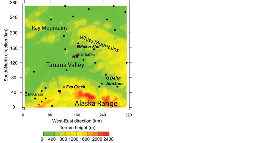
Figure 10. Topography as used in the model simulations. The black crosses, blue, red and black dots indicate the sparsely distributed radiosonde, SODAR, aerosol and meteorological sites, respectively. The open circles indicate Delta Junction, Eva Creek, and Poker Flat.
An extensive evaluation of the WRF/Chem simulations, however, was performed by Mölders et al. [20] using meteorological observations carried out at 23 sites (Figure 10). For these sites data of hourly 2 m-temperature, 2 m-dewpoint temperature, and 10 m-wind speed were available provided by the Western Region Climate Center. Also, at two sites, sea level pressure (SLP), and at 20 sites, 24 h-accumulated solar radiation were available. In their assessment of the WRF/Chem data, Mölders et al. [20] evaluated the root mean square error (RMSE), bias (simulated-observed), correlation, and standard deviation of the meteorological quantities. On average over all 23 surface meteorological sites, WRF/Chem captured the temporal evolution of the meteorological quantities well (Figure 11). Discrepancies between simulated and observed meteorological quantities occurred due to mistiming of frontal passages and after sudden strong temperature changes. On average over the entire winter period 2008/2009 and all 23 sites, the temperature, dew-point temperature, SLP, wind-speed and direction biases were 1.3 K, 2.1 K, −1.9 hPa, 1.55 m/s, and −4˚, respectively.
WRF/Chem overestimated the variance and magnitude of wind speed leading to correlations less than 0.6 in all months and 0.573 over the entire winter period. It failed to capture the high frequency of calm winds (<1 m∙s−1), but forecasted wind speed and its variance best for January, the calmest month. WRF/Chem had also difficulties in predicting wind direction, but acceptably captured its variance in all months. It provided a slightly too high (low) probability of wind-direction between 30˚ and 100˚ (140˚ and 220˚) due to terrain differences between the model and the real world. Like other meteorological models, WRF/Chem uses the mean terrain-height within a gridcell and ignores subgrid-scale terrain heterogeneity that is inherent to the observations.
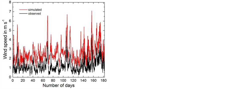
Figure 11. Time series of the simulated and observed wind speed for the winter period 2008/2009 averaged over all sites for which data were available (adopted from Mölders et al. [20]).
It is well known that models have difficulty simulating calm winds accurately. Zhao et al. [69] already reported that WRF had difficulty reproducing weak surface winds (<1.5 m∙s−1) in their long-term 4 km-increment simulation over California. This difficulty led to bias of more than 3.0 m∙s−1 and an RMSE of more than 4.5 m∙s−1. The wind data used in our study only have a bias of 1.55 m∙s−1 and an RMSE 2.4 m∙s−1 [20]. Thus, these wind speed forecasts have to be assessed as good.
Note that in the interest of focus only the quality of the wind forecasts was discussed. The interested reader can find details on the other meteorological fields and chemistry performance of WRF/Chem in [20].
Figure 12 illustrates the time series of the simulated wind speed for Delta Junction, Eva Creek, and Poker Flat over the entire period winter period 2008/2009. These results show a strong variation of wind speed. As mentioned before, the simulated wind speeds for the Eva Creek site were already used by Hinzman and Kramm [14] to predict the variation of electrical power (Figure 5) on an hourly basis. Beside these Eva Creek data, the wind speeds for Delta Junction and Poker Flat, also predicted on an hourly basis, are considered in our analysis. In addition to the wind turbine REpower MM92 (CCV) installed at the Eva Creek site, four wind turbines of other manufacturers were considered for the purpose of comparison. The specifications of each turbine are listed in Table2
4. Data Analysis
The predicted wind field data considered here are representative for heights between 64 and 113 m above ground level. The five different wind turbines chosen for our study are well within this height range. These wind field data were analyzed using a Weibull two-parameter distribution [70],
 , (4.1)
for fitting actual wind speed distributions with a minimal amount of error [71]. Here, f(v) is the probability density function of a given wind speed v occurring during a certain period of time. The quantities k and c represent the shape and scale parameters, respectively (e.g., [16,71,72]). The scale factor has units of speed and is closely related to the mean wind speed . The shape parameter is a non-dimensional quantity and is inversely related to the variance of the wind speed about the mean wind speed (e.g., [71]). The shape and scale parameters were calculated for each of the three locations (see [12,68]). The values of these parameters are listed in Table 3 and the corresponding distributions are illustrated in Figure 13. Based on the scale parameter, we have to assess the
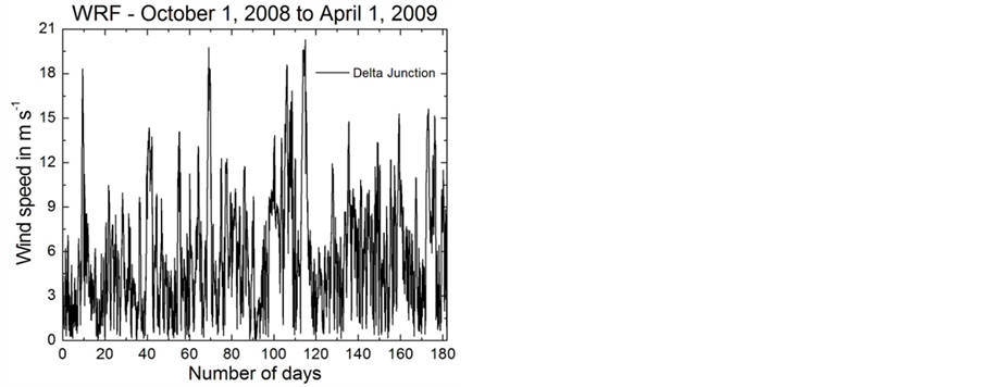
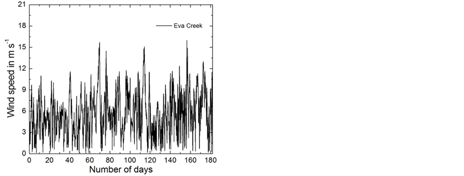
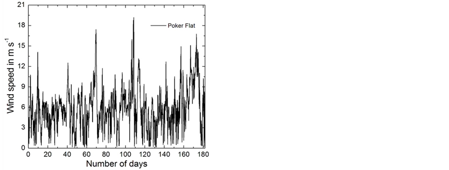
Figure 12. Hourly wind field data predicted by WRF for three locations in Interior Alaska, Delta Junction, Eva Creek, and Poker Flat, for the winter period 2008/2009. The wind data are representative for heights between 64 and 113 m above ground level. The data are taken from Mölders et al. [20].
source potential as fair. Note that the derivative of Equation (1.1) with respect to the wind speed results in , where f(v) is a function similar to Equation (4.1). This was the reason why Hinzman and Kramm [14] used the sigmoidal function (1.1) to match the power curve of the wind turbine REpower MM92.
As mentioned before, the first-order weather station Big Delta is approximately 14 km north-northeast of Delta Junction, and the small scale wind farm of AEP/ EPS is located approximately 7 km east of Delta Junction. Because of the lack of a better opportunity, we compared the Weibull shape and scale parameters for both the simulated data for Big Delta and the Delta Junction wind farm with the observational data of Big Delta. For estimating the wind speed at the hub height of 80 m at Big Delta the power law (e.g., [73,74])
 (4.2)
(4.2)
is used, where  is the mean horizontal wind speed at hub height,
  is the mean horizontal wind speed at the reference level of
  at which the measurements are performed, and the exponent
  is ranging between
  and
and .
.
Obviously, this power law does not explicitly depend on thermal stratification. In contrast to Equation (4.2), the vertical profile function of the mean horizontal wind speed (e.g., [74-77])
 (4.3)
(4.3)
demonstrates such a dependency. Here, 
is the friction velocity,  is the friction stress vector invariant with height,
  ,
,  , and
, and  are the components of the wind vector with respect to a Cartesian coordinate frame,
  is the (aerodynamic) roughness length, and
  is Panofsky’s integral similarity function for momentum defined by [75,77]
 , (4.4)
where  is the local similarity function for momentum according to Monin and Obukhov [78] related to the non-dimensional shear of the mean horizontal wind speed by
 . (4.5)
Here,  is the Obukhov number,
  is the Obukhov stability length given by
 , (4.6)
 is the von Kármán constant, g is the acceleration of
Table 2 . Specifications of the wind turbines selected for comparison in this study (adopted from Ross and Kramm [68]).
1REpower Systems SE. http://www.repower.de/fileadmin/download/produkte/PP_MM92_uk.pdf. Retrieved: July 18, 2012; 2Mitsubishi Heavy Industries, Ltd. http://www.mpshq.com/products/wind_turbines/pdf/MWT95_24.pdf. Retrieved: July 18, 2012; 3Clipper Windpower Plc. http://www.clipperwind.com/pdf/liberty_brochure.pdf. Retrieved: July 18, 2012; 4Gamesa Wind. http://www.iberdrolarenewables.us/deerfield/Zimmerman/DFLD-JZ-Rev5a-GamesaBrochure.pdf. Retrieved: July 18, 2012; 5Siemens Wind Power. http://www.energy.siemens.com/mx/pool/hq/power-generation/wind-power/E50001-W310-A102-V6-4A00_WS_ SWT-2.3-93_US.pdf. Retrieved: July 18, 2012.
Table 3. Weibull shape (k) and scale (c) parameters, according to Equation (4.1), for three locations in Interior Alaska. These parameters are based on hourly wind speed field data predicted by WRF/Chem for the winter period 2008/2009 (adopted from Ross and Kramm [68]).
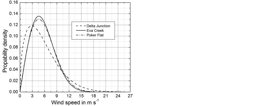
Figure 13. Weibull distributions for three locations in Interior Alaska based on the wind data illustrated in Figure 11. The corresponding shape and scale parameters are listed in Table 3 (adopted from Ross and Kramm [68]).
gravity,  is a potential temperature representative for the layer under study,
  is the vertical component of the sensible heat flux,
  is the vertical component of the water vapor flux, and
  is the specific heat at constant pressure for dry air. Note that Janjić’s [61] parameterization scheme for the ASL used in WRF is based on Monin-Obukhov similarity. If we assume that
  given by Equation (4.2) is equal to that expressed by Equation (4.3), then the exponent
  will depend explicitly on thermal stability expressed by [79]
 . (4.7)
Unfortunately, the routine measurements performed at Big Delta do not allow any determination of . Since the wind-speed data at Big Delta were only available as daily averages, also daily averages of the simulated data were generated for the purpose of comparison. These differences may contribute to the discrepancy between the Weibull parameters k and c for the Delta Junction and Big Delta illustrated in Figure 14.
Additionally, power curves for five different wind turbines were taken from the manufacturers’ websites (see Table 2). These curves give information about the power output of the turbine at a given wind speed and illustrate the cut-in wind speed, the cut-out wind speed, and rated wind speed. The power curves were determined by taking discrete values from the power curves provided by the manufacturers. Based on these discrete values, the parameters ,
,  ,
,  ,
,  ,
,  , and
, and  of the generalized logistic function (GLF),
 , (4.8)
were numerically determined for each of the five wind turbines. The function  represents the power generated by the corresponding wind turbine at the wind speed
 . A typical example obtained for the wind turbine REpower MM92 is shown in Figure 15. In this figure also the sigmoidal function (1.1) used by Hinzman and Kramm [14] is illustrated for comparison. Obviously, the GLF matches the discrete points even better. The power curves of the five wind turbines considered here are illustrated in Figure 16; the corresponding parameter values are listed in Table5
The calculations described above yielded three wind speed distributions, represented by the Weibull function
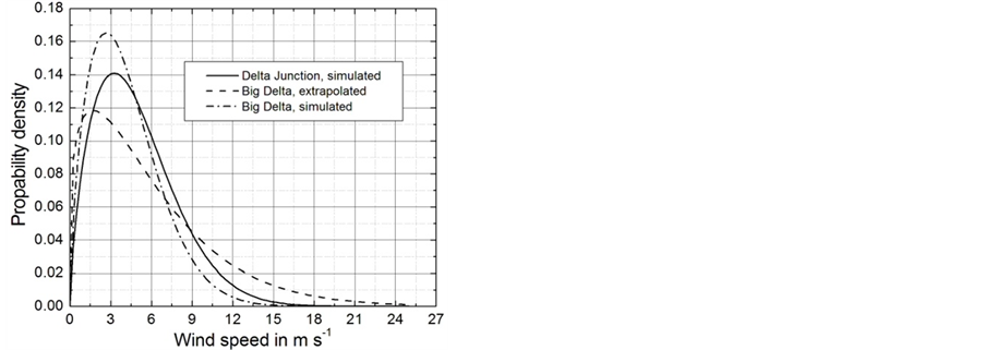
Figure 14. Weibull distributions for Delta Junction and Big Delta determined on the basis of daily mean wind speed. The corresponding shape and scale parameters are listed in Table4
Table 4. Weibull shape (k) and scale (c) parameters, according to Equation (4.1), for Delta Junction and Big Delta determined on the basis of daily mean wind speed for the winter period 2008/2009 (adopted from Ross and Kramm [68]).
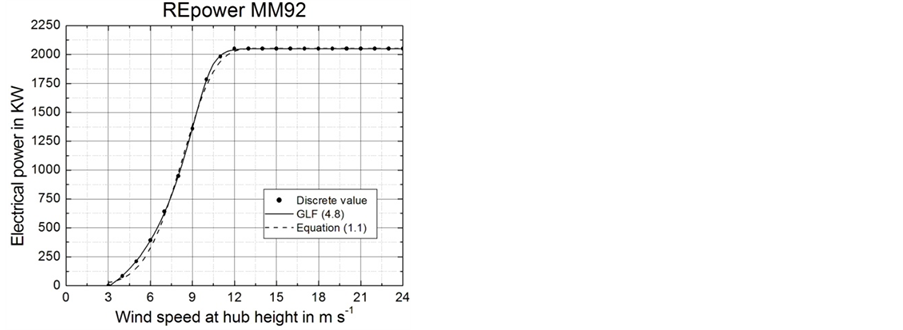
Figure 15. Power curve of the wind turbine REpower MM92. The dots show discrete values taken from the manufacturer’s information, and the solid line represents the GLF, where its parameters listed in Table 4 were determined on the basis of these discrete values (adopted from Ross and Kramm [68]). Also illustrated is the sigmoidal function (1.1).
(4.1), and five power curves, represented by the GLF (4.8). For a known probability distribution  and the power curve
 , the average power output can be estimated by the integration (e.g., [56,71])
 (4.9)
(4.9)
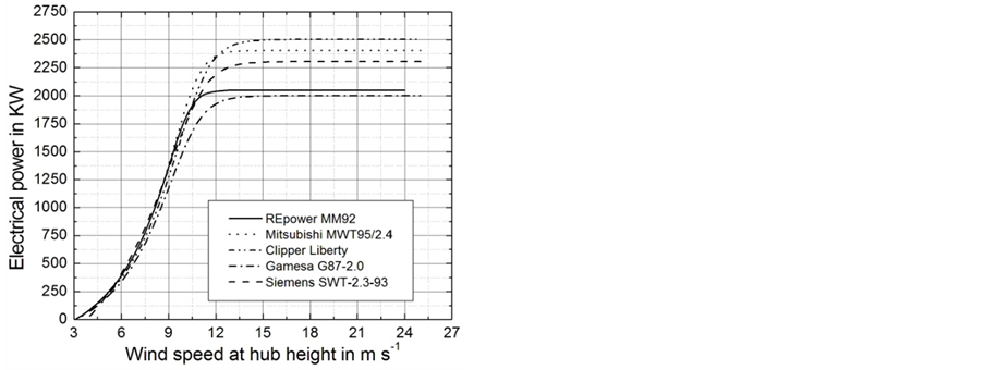
Figure 16. Power curves of the wind turbines considered in this study. They are based on the parameters of the GLF listed in Table 5 (adopted from Ross and Kramm [68]).
Table 5. Parameters A, K, Q, B, M, and u of the generalized logistic function (4.8) used to model the wind turbines’ power curves (adopted from Ross and Kramm [68]).
that covers the range from the cut-in wind speed to the cut-out wind speed of each of the wind turbines. This average power output can be used to calculate the capacity factor,  , of each wind turbine at each location using the formula
 , (4.10)
where  is the rated power of any turbine [56]. The rated power of each turbine is illustrated in Figure 16. The results provided by Equations (4.9) and (4.10) were used to analyze which location would yield the most power for the period under study and which wind turbine would be the best for each location.
5. The Predicted Wind Power
Results of the predicted wind power and the corresponding capacity factor are illustrated in Figures 17 and 18, respectively. As shown in Figure 17, the wind power potential at Delta Junction and Poker Flat is slightly better that of the Eva Creek site, where the type of the wind turbine chosen can notably influence the power generation at a given location. Based on the results of the predicted wind fields, the Mitsubishi wind turbine would produce the most power at all three locations. This is due to the fact that the wind speed at which the rated power is
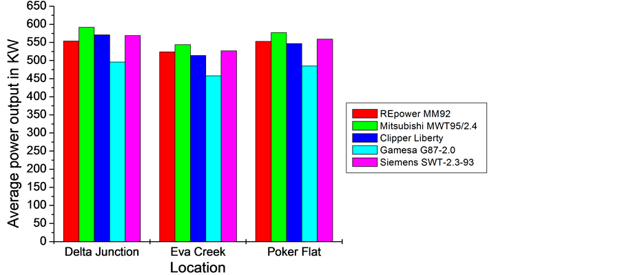
Figure 17. Predicted average power output as provided by Equation (4.9) for three locations in Interior Alaska with respect to the winter period 2008/2009 (adopted from Ross and Kramm [68]).
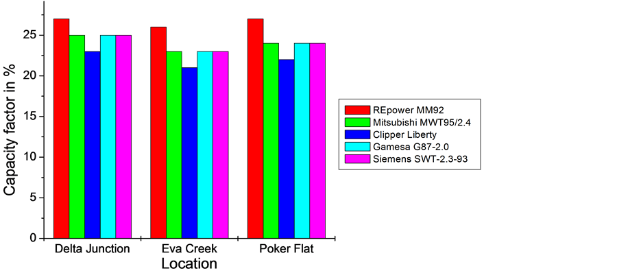
Figure 18. Predicted capacity factor as provided by Equation (4.10) for three locations in Interior Alaska with respect to the winter period 2008/2009 (adopted from Ross and Kramm [68]).
achieved is relatively low (rated speed: 12.5 m∙s−1) and that it has the largest swept area of the five turbines (see Table 2). On the contrary, the Gamesa wind turbine would produce the lowest power output at all three locations. It has not only the lowest swept area of the five wind turbines, but also the highest rated speed of 17 m∙s−1. Whereas the wind turbines of REpower, Clipper, and Siemens would provide similar power output. Note that in case of REpower MM92 our values of the average power output for Eva Creek is slightly higher than that reported by Hinzman and Kramm [14] (see Figure 5).
If we assess the capacity factor, the picture will be different. As shown in Figure 18, the REpower MM92 has the highest capacity factor for all three locations, meaning it would utilize the wind more effectively than all other ones. The capacity factors of the wind turbines of Mitsubishi, Gamesa, and Siemens are identical and notably higher than that of Clipper.
The capacity factor of the 12 REpower wind turbines installed at the Eva Creek site is illustrated in Figure 19 for the period January to September 2013. It amounts to 31 percent, on average, for this period. This value is notably higher than our predicted capacity factor, but also notably lower than the average annual capacity factor 36% assumed by GVEA. From the statistics of the GVEA’s Healy Wind Demonstration Project that was in service from September 10, 1998 to October 14, 2000, we may infer that the mean monthly wind speed is highly variable in the Healy area (Figure 20). This might be the reason why our prediction for the winter period October 1, 2008, to April 1, 2009 is nearly 20 percent lower than the capacity factor of the EVA Creek wind farm in 2013.
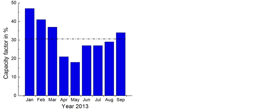
Figure 19. Time series of the capacity factor of the Eva Creek wind farm (data taken from the GVEA’s website http://www.gvea.com/energy/evacreek/output).
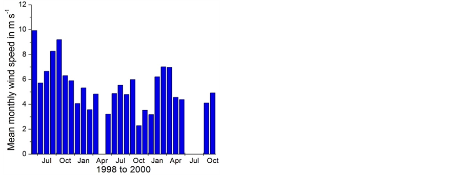
Figure 20. Time series of the mean monthly wind speed (data taken from GVEA’s Summary of the Healy Wind Demonstration Project, September 19, 2002). Note that no data were available for April 1999 and June to August 2000.
It would be advantageous and reasonable to use the meteorological towers at the Eva Creek site for further evaluation purposes, but these data are classified as confidential. The same is true in case of the small scale wind farm at Delta Junction. Such data are also indispensable for analyzing the ramp power structure at a given site (e.g., [80]).
6. Final Remarks and Conclusions
In our study, we assessed the wind power potential in Interior Alaska for the winter period 2008/2009 from a micrometeorological perspective. Based on the local balance equation of momentum and the equation of continuity we derived the local balance equation of kinetic energy for macroscopic and turbulent systems to outline the generation of electricity by extracting kinetic energy from the wind field. In a further step, also Bernoulli’s equation and integral equations were presented that customarily serve as the key equations in momentum theory and blade-element analysis. It was shown that not only molecular, but also turbulent effects are usully ignored in deriving these equations. Results of the Lanchester-BetzJoukowsky limit, Glauert’s optimum actuator disk, and the blade-element analysis by Okulov and Sørensen were exemplarily illustrated.
The use of wind power may not only serve to reduce the consumption of fossil fuel to generate electricity, but may also contribute to solving the air quality issue in the Fairbanks area. For our study we used WRF/Chem predictions to avoid time-consuming and expensive talltower observations at different locations in Interior Alaska. To predict the power output we used Weibull distributions derived from the predicted wind fields for these three sites and the power curves of the five different wind turbines with rated powers ranging from 2 MW to 2.5 MW, where these power curves are represented by general logistic functions. The predicted power capacity for the Eva Creek site was compared with that of the Eva Creek wind farm installed in 2012.
Based on our wind power predictions for three locations in Interior Alaska and five different wind turbines, we found that the wind power potential at Delta Junction and Poker Flat is slightly higher than that at the Eva Creek site. This means that the Delta Junction site is suitable for installing a second wind farm of 25 MW rated power as proposed by AEP/EPS. A wind turbine installed at Poker Flat could help reduce University of Alaska’s costs in running the Poker Flat Research Range. We also found that the type of the wind turbine chosen can notably influence the power generation at a given location. Our results suggest that the wind turbine REpower MM92 has the highest capacity factor of the five wind turbines considered in our study. Compared with the results of the Eva Creek wind farm for the period January to September 2013, the results of our predictions for the winter period 2008/2009 are nearly 20 percent lower. This result may be attributed to the fact that the mean monthly wind speed is highly variable in the Healy area.
A second wind farm would be desirable to fulfill GVEA’s Renewable Energy Pledge and to mitigate the air pollution in Fairbanks. As reported by GVEA, during the period from January to March 2013, the electricity generated by the Eva Creek wind farm served to power more than 10250 average Interior homes (based on 660 kWh per month) for each month.
However, the wintertime conditions in Interior Alaska with near-surface air temperatures of  and even notably lower do not allow the use of wind power without spinning reserve that covers, at least, one-third of the rated power of a wind farm. The spinning reserve is intended to protect the system against unforeseen events such as generation outages, sudden load changes or a combination of both (e.g., [81]).
It is quite understandable that spinning reserve causes costs. As already pointed out by Ortega-Vazquez and Kirschen [81], the costs of spinning reserve are far from negligible. If larger amounts of spinning reserve must be scheduled because of a higher wind-power penetration, then a larger number of conventional generating units will need to be synchronized.
Modern heating systems as installed for the economical use of liquid fuel under cold climate conditions require electricity for controlling and regulating. This means that a generation outage for several hours or even days is unacceptable because it would be life-threatening for human beings, livestock, and pet animals.
Consequently, the use of wind power in Interior Alaska must be backed up by conventional power plants at all costs. These power plants idling in the background must be ready to generate electricity immediately for compensating the loss of wind power due to unfavorable weather conditions. According to John Sloan, secretary of the GVEA Board of Directors [82], “GVEA’s system has adequate backup capacity for Eva Creek, but adding more wind would require the co-op to keep multiple oil-fired power plants idling in the background, burning lots of oil but producing little power”.
Natural gas power plants would be preferable as standby power plants. Unfortunately, natural gas is not available in Interior Alaska in sufficient quantity. Thus, liquid fuel (and/or coal) power plants have to be considered. These power plants need some time to achieve the optimum of their operating states. Consequently, reliable weather forecasts for Interior Alaska for, at least, 48 hours will be indispensable to timely cover the loss of wind power due to unfavorable weather situations which include not only light wind periods, but also those that can cause icing if the rotor blades are hit by super-cooled water. In case of icing a shutdown of wind turbines is inevitable. According to Ortega-Vazquez and Kirschen [81], accurate wind power predictions may support grid operators to schedule appropriate levels and types of operating reserves needed to perform the different regulation tasks. Such wind power predictions were outlined by Hinzman and Kramm [14] on the basis of predicted wind fields. These authors used an hourly basis, but shorter periods can be considered.
A wind turbine acts as a sink of kinetic energy transported by the wind field. As the Eva Creek wind farm consists of sparsely distributed turbines, this aerodynamic effect might be negligible. In case of larger wind farms it may become important. Thus, there is an urgent need to parameterize this divergence effect in mesoscale numerical models of the atmosphere if they are to be considered to predict the electricity generated by larger wind farms. It may be carried out by considering the wind power density related to the power curve of the wind turbine.
Based on our findings we may conclude that the decision of GVEA to install the cold climate version of REpower’s wind turbine MM92 at the Eva Creek site was reasonable. Nevertheless, other aspects outside the scope of this micrometeorological study have to be assessed when choosing the best wind turbine for a specific site. These may be, for instance, the cost and the maintenance intervals of the wind turbine.
Acknowledgements
We would like to express much gratitude to the National Science Foundation for funding the project work of Megan Hinzman and Samuel Smock in summer 2011, and Hannah K. Ross and John Cooney in summer 2012 through the Research Experience for Undergraduates (REU) Program, grant number AGS1005265. We also would like to extend gratitude to the Alaska Department of Labor for funding Dr. Gary Sellhorst’s project work.
REFERENCES
- T. Godish, “Air Quality,” Lewis Publishers, Boca Raton, 2004.
- F. Dominici, R. D. Peng, M. L. Bell, L. Pham, A. McDermott, S. L. Zeger and J. M. Samet, “Fine Particulate Air Pollution and Hospital Admission for Cardiovascular and Respiratory Diseases,” JAMA, Vol. 295, No. 10, 2006, pp. 1127-1134. http://dx.doi.org/10.1001/jama.295.10.1127
- K. A. Miller, D. S. Siscovick, L. Sheppard, K. Shepherd, J. H. Sullivan, G.L. Anderson and J. D. Kaufman, “LongTerm Exposure to Air Pollution and Incidence of Cardiovascular Events in Women,” New England Journal of Medicine, Vol. 356, No. 5, 2007, pp. 447-458. http://dx.doi.org/10.1056/NEJMoa054409
- R. J. Delfino, S. Brummel, J. Wu, H. Stern, B. Ostro, M. Lipsett, A. Winer, D. H. Street, L. Zhang, T. Tjoa and D. L. Gillen, “The Relationship of Respiratory and Cardiovascular Hospital Admissions to the Southern California Wildfires of 2003,” Occupational & Environmental Medicine, Vol. 66, No. 3, 2009, pp. 189-197. http://dx.doi.org/10.1136/oem.2008.041376
- J. Schwartz, D. Dockery and L. Neas, “Is Daily Mortality Associated Specifically with Fine Particles?” Journal of the Air & Waste Management Association, Vol. 46, No. 10, 1997, pp. 927-939. http://dx.doi.org/10.1080/10473289.1996.10467528
- S. M. Bernard, J. M. Samet, A. Grambsch, K. L. Ebi and I. Romieu, “The Potential Impacts of Climate Variability and Change on Air Pollution Related Health Effects in the United States,” Environmental Health Perspectives, Vol. 109, Suppl. 2, 2001, pp. 199-209.
- A. D. Kappos, P. Bruckmann, T. Eikmann, N. Englert, U. Heinrich, P. Höppe, E. Koch, G. H. M. Krause, W. G. Kreyling, K. Rauchfuss, P. Rombout, V. Schulz-Klemp, W. R. Thiel and H. E. Wichmann, “Health Effects of Particles in the Ambient Air,” International Journal of Hygiene and Environmental Health, Vol. 207, No. 4, 2004, pp. 399- 407. http://dx.doi.org/10.1078/1438-4639-00306
- H. N. Q. Tran and N. Mölders, “Investigations on Meteorological Conditions for Elevated PM2.5 in Fairbanks, Alaska,” Atmospheric Research, Vol. 99, No. 1, 2011, pp. 39-49. http://dx.doi.org/10.1016/j.atmosres.2010.08.028
- Committee on Carbon Monoxide Episodes in Meteorological and Topographical Problem Areas, National Research Council, “The Ongoing Challenge of Managing Carbon Monoxide Pollution in Fairbanks, Alaska,” Interim Report, National Academy of Sciences, 2002.
- N. Mölders and G. Kramm, “A Case Study on Wintertime Inversions in Interior Alaska with WRF,” Atmospheric Research, Vol. 95, No. 2-3, 2010, pp. 314-332. http://dx.doi.org/10.1016/j.atmosres.2009.06.002
- G. Wendler and M. Shulski, “A Century of Climate Change for Fairbanks, Alaska,” Arctic, Vol. 62, No. 3, 2009, pp. 295-300.
- J. Cooney and G. Kramm, “Determining Viable Locations for Wind Farms in Alaska,” NSF REU Site Program in Atmospheric Sciences, University of Alaska Fairbanks, Geophysical Institute, Fairbanks, Alaska, 2012.
- B. Newton and G. Wyman, “Eva Creek Briefing,” Golden Valley Electrical Association, 2012.
- M. Hinzman and G. Kramm, “The Eva Creek Wind Farm project,” NSF REU Site Program in Atmospheric Sciences, University of Alaska Fairbanks, Geophysical Institute, Fairbanks, Alaska, 2011.
- B. Storm, J. Dudhia, S. Basu, A. Swift and I. Giammanco, “Evaluation of the Weather Research and Forecasting Model on Forecasting Low-Level Jets: Implications for Wind Energy,” Wind Energy, Vol. 12, No. 1, 2009, pp. 81-90. http://dx.doi.org/10.1002/we.288
- B. Storm and S. Basu, “The WRF Model Forecast-Derived Low-Level Wind Shear Climatology over the United States Great Plains,” Energies, Vol. 3, No. 2, 2010, pp. 258-276. http://dx.doi.org/10.3390/en3020258
- W. C. Skamarock, J. B. Klemp, J. Dudhia, D. O. Gill, D. M. Barker, M. G. Duda, X.-Y. Huang, W. Wang and J. G. Powers, “A Description of the Advanced Research WRF Version 3,” NCAR Technical Note, NCAR/TN-475+STR, Colorado, 2008.
- N. Mölders, H. N. Q. Tran, P. Quinn, K. Sassen, G. E. Shaw and G. Kramm, “Assessment of WRF/Chem to Capture Sub-Arctic Boundary Layer Characteristics during Low Solar Irradiation Using Radiosonde, SODAR, and Surface Data,” Atmospheric Pollution Research, Vol. 2, 2011, pp. 283-299.
- G. Kramm, G. Sellhorst, H. K. Ross, J. Cooney, R. Dlugi and N. Mölders, “On the Maximum of Wind Power Efficiency,” 2013 (prepared for submission).
- N. Mölders, H. N. Q. Tran, C. F. Cahill, K. Leelasakultum and T. T. Tran, ”Assessment of WRF/Chem PM2.5- Forecasts Using Mobile and Fixed Location Data from the Fairbanks, Alaska Winter 2008/09 Field Campaign,” Atmospheric Pollution Research, Vol. 3, No. 2, 2012, pp. 180-191.
- S. R. de Groot and P. Mazur, “Non-Equilibrium Thermodynamics,” North-Holland Publishing Comp, Amsterdam/ London, 1969.
- L. D. Landau and E. M. Lifshitz, “Course of Theoretical Physics-Vol. 6, Fluid Mechanics,” 2nd Edition, Pergamon Press, Oxford, New York, Toronto, Sydney, Paris, Frankfurt, 1987.
- O. Reynolds, “On the Dynamical Theory of Incompressible Viscous Fluids and the Determination of the Criterion,” Philosophical Transactions of the Royal Society, Vol. 186, 1895, pp. 123-164. http://dx.doi.org/10.1098/rsta.1895.0004
- G. Kramm and F. X. Meixner, “On the Dispersion of Trace Species in the Atmospheric Boundary Layer: A Re-Formulation of the Governing Equations for the Turbulent Flow of the Compressible Atmosphere,” Tellus, Vol. 52, No. 5, 2000, pp. 500-522. http://dx.doi.org/10.1034/j.1600-0870.2000.00984.x
- R. B. Montgomery, “Convection of Heat,” Archiv für Meteorologie, Geophysik und Bioklimatologie, Serie A, Vol. 7, No. 1, 1954, pp. 125-132. http://dx.doi.org/10.1007/BF02277911
- H. Fortak, “Zur Energetik der Planetarischen Grenzschicht,” Annalen der Meteorologie (NF), Vol. 4, 1969, pp. 157-162.
- H. Pichler, “Dynamik der Atmosphäre,” Bibliographisches Institut, Zürich, 1984.
- G. Cox, “Basic Considerations,” In: G. Cox, Ed., Combustion Fundamentals of Fire, Academic Press, London, San Diego, New York, pp. 3-30.
- G. Kramm, R. Dlugi and D. H. Lenschow, “A Re-Evaluation of the Webb-Correction Using Density-Weighted Averages,” Journal of Hydrology, Vol. 166, No. 3-4, 1995, pp. 283-292. http://dx.doi.org/10.1016/0022-1694(94)05088-F
- D. Thomson, “The Parameterization of the Vertical Dispersion of a Scalar in the Atmospheric Boundary Layer,” Atmospheric Environment, Vol. 29, No. 11, 1995, p. 1343. http://dx.doi.org/10.1016/1352-2310(94)00326-G
- A. Venkatram, “Response,” Atmospheric Environment, Vol. 32, No. 2, 1998, p. 259. http://dx.doi.org/10.1016/S1352-2310(96)00078-7
- A. S. Kowalski, “Exact Averaging of Atmospheric State and Flow Variables,” Journal of the Atmospheric Sciences, Vol. 69, No. 5, 2012, pp. 1750-1757. http://dx.doi.org/10.1175/JAS-D-11-0299.1
- T. Hesselberg, “Die Gesetze der Ausgeglichenen Atmosphärischen Bewegungen,” Beitr. Phys. fr. Atmosph., Vol. 12, No. 3, 1926, pp. 141-160.
- J. van Mieghem, “Les Equations Générales de la Mécanique et de L’Energétique des Milieux Turbulents en vue des Applications à la Météorologie,” Institut Royal Météorologique de Belgique, Belgique., Mém. XXXIV, 1949.
- J. van Mieghem, “Atmospheric Energetics,” Clarendon Press, Oxford, 1973.
- F. Herbert, “Irreversible Prozesse der Atmosphäre-3. Teil (Phänomenolo-gische Theorie Mikroturbulenter Systeme),” Beitr. Phys. Atmosph, Vol. 48, No. 1, 1975, pp. 1-29. (in German).
- P. A. Libby and F. A. Williams, “Turbulent Reacting Flows,” Springer-Verlag, Berlin, 1980. http://dx.doi.org/10.1007/3-540-10192-6
- F. Herbert, “A Re-Evaluation of the Webb Correction Using Density-Weighted Averages-Comment,” Journal of Hydrology, Vol. 173, No. 1-4, 1995, pp. 343-344. http://dx.doi.org/10.1016/0022-1694(95)02867-O
- A. Eliassen and E. Kleinschmidt Jr., “Dynamic Meteorology,” In: S. Flügge, Ed., Handbuch der Physik, Bd. XLVIII, Springer-Verlag Berlin, Heidelberg, New York, 1957, pp. 1-154.
- J. A. Dutton, “Dynamics of Atmospheric Motion,” Dover, New York, 1995.
- J. C. Rotta, “Turbulente Strömungen,” B.G. Teubner, Stuttgart, 1972. http://dx.doi.org/10.1007/978-3-322-91206-0
- D. Hilbert and S. Cohn-Vossen, “Geometry and the Imagination,” Chelsea Publishing, New York, 1952.
- A. Budó, “Theoretische Mechanik,” VEB Deutscher Verlag der Wissenschaften, Germany, 1990.
- S. V. Alekseenko, P. A. Kuibin and V. L. Okulov, “Theory of Concentrated Vortices,” Springer, Berlin, Heidelberg, New York, 2007.
- J. N. Sørensen, “Aerodynamic Aspects of Wind Energy Conversion,” Annual Review of Fluid Mechanics, Vol. 43, 2011, pp. 427-448.
- P. M. Goorjian, “An Invalid Equation in the General Momentum Theory of the Actuator Disk,” AIAA Journal, Vol. 10, No. 4, 1972, pp. 543-544.
- R. E. Wilson and P. B. S. Lissaman, “Applied Aerodynamic Performance of Wind Power Machines,” Oregon State University, Corvallis, 1974.
- G. A. M. van Kuik, “The Lanchester-Betz-Joukowsky Limit,” Wind Energy, Vol. 10, No. 3, 2007, pp. 289-291.
- V. L. Okulov and J. N. Sørensen, “Refined Betz Limit for Rotors with a Finite Number of Blades,” Wind Energy, Vol. 11, No. 4, 2008, pp. 415-426.
- A. Betz, “Wind-Energie und Ihre Ausnutzung Durch Windmühlen,” Vandenhoeck & Ruprecht, Göttingen, 1926.
- W. J. M. Rankine, “On the Mechanical Principles of the Action of Propellers,” Transaction of the Institute of Naval Architects, Vol. 6, 1865, pp. 13-39.
- W. Froude, “On the Elementary Relation between Pitch, Slip and Propulsive Efficiency,” Transaction of the Institute of Naval Architects, Vol. 19, 1878, pp. 22-33.
- R.E. Froude, “On the Part Played in Propulsion by Difference in Pressure,” Transaction of the Institute of Naval Architects, Vol. 30, 1889, pp. 390-405.
- H. Snel, “Review of the Present Status of Rotor Aerodynamics,” Wind Energy, Vol. 1, No. S1, 1998, pp. 46-69.
- V. L. Okulov and J. N. Sørensen, “Maximum Efficiency of Wind Turbine Rotors Using Joukowsky and Betz Approaches,” Journal of Fluid Mechanics, Vol. 649, 2010, pp. 497-508. http://dx.doi.org/10.1017/S0022112010000509
- S. Mathew, “Wind Energy: Fundamentals, Resource Analysis, and Economics,” Springer, Berlin, Heidelberg, New York, 2006. http://dx.doi.org/10.1007/3-540-30906-3
- H. Glauert, “Airplane Propellers,” In: W. F. Durand, Ed., Aerodynamic Theory, Vol. IV, Division L, Springer, New York, 1935, pp. 169-360.
- S.-Y. Hong and J.-O. J. Lim, “The WRF Single-Moment 6-Class Microphysics Scheme (WSM6),” Journal of the Korean Meteorological Society, Vol. 42, No. 2, 2006, pp. 129-151.
- G. A. Grell and D. Devenyi, “A Generalized Approach to Parameterizing Convection Combining Ensemble and Data Assimilation Techniques,” Geophysical Research Letters, Vol. 29, No. 14, 1693, pp. 1-4. http://dx.doi.org/10.1029/2002GL015311
- E. J. Mlawer, S. J. Taubman, P. D. Brown, P.D., M. J. Iacono and S. A. Clough, “Radiative Transfer for Inhomogeneous Atmospheres: RRTM, a Validated CorrelatedK Model for the Longwave,” Journal of Geophysical Research: Atmospheres, Vol. 102, No. D14, 1997, pp. 16663-16682.
- Z. I. Janjić, “Nonsingular Implementation of the MellorYamada Level 2.5 Scheme in the NCEP Meso Model,” National Centers for Environmental Prediction (NCEP) Office Note #437, 2002.
- T. G. Smirnova, J. M. Brown, S. G. Benjamin and D. Kim, “Parameterization of Cold-Season Processes in the MAPS Land-Surface Scheme,” Journal of Geophysical Research: Atmospheres, Vol. 105, No. D3, 2000, pp. 4077-4086.
- W. R. Stockwell, P. Middleton, J. S. Chang and X. Tang, “The Second Generation Regional Acid Deposition Model Chemical Mechanism for Regional Air Quality Modeling,” Journal of Geophysical Research: Atmospheres, Vol. 95, No. D10, 1990, pp. 16343-16367.
- S. Madronich, “Photodissociation in the Atmosphere. 1. Actinic Flux and the Effects of Ground Reflections and Clouds,” Journal of Geophysical Research: Atmospheres, Vol. 92, No. D8, pp. 9740-9752.
- M. L. Wesely, “Parameterization of Surface Resistances to Gaseous Dry Deposition in Regional Scale Numerical Models,” Atmospheric Environment, Vol. 23, No. 6, 1989, pp. 1293-1304.
- I. J. Ackermann, H. Hass, M. Memmesheimer, A. Ebel, F. S. Binkowski and U. Shankar, “Modal Aerosol Dynamics Model for Europe: Development and First Applications,” Atmospheric Environment, Vol. 32, No. 17, 1998, pp. 2981-2999.
- B. Schell, I. J. Ackermann, H. Hass, F. S. Binkowski and A. Ebel, “Modeling the Formation of Secondary Organic Aerosol within a Comprehensive Air Quality Model System,” Journal of Geophysical Research: Atmospheres, Vol. 106, No. D22, pp. 28275-28293.
- H. Ross and G. Kramm, “An Assessment of Wind Power Potential for Interior Alaska,” NSF REU Site Program in Atmospheric Sciences, University of Alaska Fairbanks, Geophysical Institute, Fairbanks, Alaska, 2012.
- Z. Zhao, S. H. Chen, M. J. Kleeman, M. Tyree and D. Cayan, “The Impact of Climate Change on Air Quality-Related Meteorological Conditions in California. Part I: Present Time Simulation Analysis,” Journal of Climate, Vol. 24, No. 13, 2011, pp. 3344-3361.
- W. Weibull, “A Statistical Distribution Function of Wide Applicability,” Journal of Applied Mechanics, Vol. 18, 1951, pp. 293-297.
- C. G. Justus, W. R. Hargraves and A. Yalcin, “Nationwide Assessment of Potential Output from Wind-Powered Generators,” Journal of Applied Meteorology, Vol. 15, No. 7, 1976, pp. 673-678.
- K. Ulgen and A. Hepbasli, “Determination of Weibull Parameters for Wind Energy Analysis of Izmir, Turkey,” International Journal of Energy Research, Vol. 26, No. 6, 2002, pp. 495-506. http://dx.doi.org/10.1002/er.798
- G. J. Haltiner and F. L. Martin, “Dynamical and Physical Meteorology,” McGraw-Hill Book Company, New York, Toronto, London, 1957.
- S. Pal Arya, “Introduction to Micrometeorology,” Academic Press, San Diego, New York, Boston, London, Sydney, Tokyo, Toronto, 1988.
- H. A. Panofsky, “Determination of Stress from Wind and Temperature Measurements,” Quarterly Journal of the Royal Meteorological Society, Vol. 89, No. 379, 1963, pp. 85-94.
- G. Kramm and F. Herbert, “Similarity Hypotheses for the Atmospheric Surface Layer Expressed by Dimensional π Invariants Analysis—A Review,” The Open Atmospheric Science Journal, Vol. 3, 2009, pp. 48-79.
- G. Kramm, D. J. Amaya, T. Foken and N. Mölders, “Hans A. Panofsky’s Integral Similarity Function—At Fifty,” Atmospheric and Climate Sciences, Vol. 3, 2013, pp. 581-594.
- A. S. Monin and A. M. Obukhov, “Osnovnye Zakonomernosti Turbulentnogo Peremešivanija v Prizemnom Sloe Atmosfery,” Trudy Geofizicheskogo Instituta, Akademiya Nauk SSSR, Vol. 24, No. 151, 1954, pp. 163-187.
- S. Smock and G. Kramm, “Power-Law and Logarithmic Wind Profiles: A Synthesis,” NSF REU Site Program in Atmospheric Sciences, University of Alaska Fairbanks, Geophysical Institute, Fairbanks, Alaska, 2011.
- Y.-H. Wan, “Wind Power Plant Behaviors: Analyses of Long-Term Wind Power Data,” National Renewable Energy Laboratory, Technical Report NREL/TP-500-36551, 2004.
- M. A. Ortega-Vazquez and D. S. Kirschen, “Estimating the Spinning Reserve Requirements in Systems with Significant Wind Power Generation Penetration,” IEEE Transactions on Power Systems, Vol. 24, No. 1, 2009, pp. 114-124.
- J. Sloan, “A Limit on Wind Power,” Fairbanks Daily News-Miner, 2013. (Community Perspective) http://www.newsminer.com/opinion/community_perspectives/a-limit-on-wind-power/article_54f7fdd0-3962-11e3-900f-0019bb30f31a.html
NOTES
*Corresponding author.