Atmospheric and Climate Sciences
Vol.3 No.1(2013), Article ID:27582,10 pages DOI:10.4236/acs.2013.31013
Seasonal Variations of the Surface Fluxes and Surface Parameters over the Loess Plateau in China
1Graduate School of Environmental Studies, Nagoya University, Nagoya, Japan
2Research Institute for Humanity and Nature, Kyoto, Japan
3Hydrospheric Atmospheric Research Center, Nagoya University, Nagoya, Japan
Email: misswindy78@gmail.com
Received July 18, 2012; revised August 20, 2012; accepted August 29, 2012
Keywords: Loess Plateau; Surface Fluxes; Bulk Transfer Coefficient; Soil Moisture Availability
ABSTRACT
Turbulent fluxes were measured by an eddy covariance system at three levels over an intricate land surface on the southern part of the Loess Plateau, consisting of heterogeneous flat terrain and a large valley 500 m away from the observation site to the southeast. The surface roughness length, the seasonal variation of bulk transfer coefficient for sensible heat (CH), and the seasonal variation of surface moisture availability (β) were also analyzed based on the observation. The flux footprint was carefully considered in this study. A relatively dry period of the experimental area existed from June to the first week of July 2004 when the land surface offered turbulent energy to the atmospheric surface layer mainly by sensible heat flux with a maximum value of around 230 Wm−2. A wet duration lasted from the second week of July to the end of September 2004 with very frequent rainfall events in conditions when the winds were mainly from the southeast;latent heat flux was dominant during the wet season and reached a peak value of around 280 Wm−2. The surface parameters of CH and β were calculated when the mean winds coming from the flat terrain, i.e., from the northwest direction. The values of CH ranged between 0.004 and 0.006 during the observational year of June 2004 to June 2005. The surface moisture availability β changed with seasons as anticipated with high values during June and July 2004 and lowest values around 0.03 in February 2005. Its peak value of 0.91 occurred in July; the mean value of β during the wet season was 0.29. Furthermore, the relationship between the surface soil water content and β indicated that changes in soil water content contributed much to variations of surface moisture availability β.
1. Introduction
Turbulent fluxes in the atmospheric surface layer (ASL) are not only governed by properties of the airflow, they are also closely connected to the structure and function of the underlying surface. Generally, land surfaces are not homogeneous; the vertical structure of the atmospheric boundary layer (ABL) is modified over heterogeneous surfaces compared with that over homogeneous surfaces. As Wyngaard [1] ever pointed out, it is always a difficult challenge to determine accurate and representative surface fluxes over heterogeneous surfaces.
The Loess Plateau in China, as a semi-arid plateau, located within the middle reaches of the Yellow River basin and being affected by the Asian monsoon activities in summer, possesses a unique heterogeneity of topography and consequently induces typical processes of energy budget and fluxes transportations in the ABL. Measuring accurate surface energy fluxes and surface parameters over the Loess Plateau have significant meanings for the ABL evolution study over such a heterogeneous landscape, the Asian monsoon and climate change studies, and the research of the water cycle systems of the Yellow River Basin and even of the Eastern Asia. The field campaign in this study which was equipped with a flux tower and a wind profile Radar was the first ABL field observation conducted over the Loess Plateau [2].
In literatures, Kimura et al. [3,4] ever studied seasonal variations of heat balance including sensible and latent heat fluxes and soil moisture on the Loess Plateau using a three-layer soil model and verified the model by observations over bare soil fields. Liu et al. [5] simulated regional evapotranspiration during 20 years by three complementary models over the Yellow River basin within which the Loess Plateau lies. These studies ignored the effects of surface heterogeneity on surface fluxes, evapotranspiration, and surface heat balance. However, many studies have been conducted to estimate the heat transfer and evapotranspiration over complex terrains utilizing synergetic methods. Tamagawa [6] obtained mean bulk transfer coefficient for sensible heat from observed flux data and mast profiles over a desert area. A multilayer energy budget model was proposed by Kondo and Watanabe [7] which indicated that the bulk transfer coefficients for sensible and latent heat were sensitive to meteorological conditions when using the radiative surface temperature as the mean surface temperature. Kafle and Yamaguchi [8] estimated the spatial distribution of evapotranspiration over an intricate topography using a topography-considered two-source energy balance model based on remote sensing data and meteorological data. Kustas et al. [9] also studied the effect of pixel resolution of the remote sensing inputs on model flux estimates for an agricultural region.
Based the ABL experiment in this study, many works have been done to investigate the effects of topography and surface heterogeneity on the ABL properties over the experimental region on the Loess Plateau. Li et al. [10] studied the characteristics of turbulent spectra when winds from the flat terrain and from the southeastern valley, and found that for flow from the valley direction the valley did significantly influence the shape of the lateral spectrum indicating the modification of the overlying ABL structure. The effect of the topography on local circulation and cumulus generation over this region was evaluated by Nishikawa et al. [11] through numerical simulations of ABL using a cloud-resolving nonhydrostatic model. Takahashi et al. [12] investigated the diurnal variation of water vapor mixing between the ABL and the free atmosphere over the Loess Plateau based on the measurements of water vapor and wind by the ground-based microwave radiometer and the wind profile Radar.
In this paper, we will estimate the surface energy fluxes over the experimental site. The main objective is to study the variability of surface fluxes with the surface wetness. The seasonal variations of the bulk transfer coefficient for sensible heat and the surface moisture availability will be presented to investigate the properties of energy transfer and evapotranspiration over the studied region on the Loess Plateau.
2. Study Area
2.1. Experimental Site
The ABL observation in this study was carried out at a field site (35˚12'N, and 107˚40'E) located in the middle southern area of the Loess Plateau in China. The Loess Plateau has a semi-arid land climate, and lies within 34˚ to 40˚N and 100˚ to 115˚E. The Loess Plateau consists generally of strongly dissected flat terrain and gullies extending long to several tens kilometers with typical depths in the order of 100 m and surface widths in the order of 1 km [10]. Its total area is 0.62 million km2 (35% tableland; 65% gully slopes). The annual precipitation ranges from 150 to 750 mm, 70% of which falls in summer. Because loess soil is susceptible to erosion, the Loess Plateau landscape includes numerous steep gullies. Approximately 90% of the soil deposited into the Yellow River each year originates from the Loess Plateau [3,4, 13].
The land cover of the studied site is heterogeneous, consisting of wheat, apple trees, and residences; the area is mainly flat, except for a large valley with the nearest edge about 500 m away from the observation tower in the southeast. The valley has the depth of around 100 m, a surface width of about 1 km, and the length around 20 km extending to the southeast (see Figure 1).
2.2. Climatology
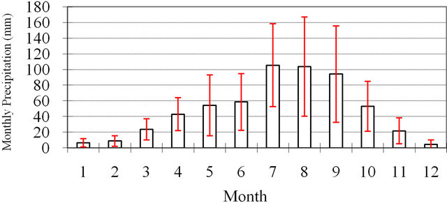
The monthly precipitation and mean air temperature averaged during 45 years from 1957 to 2001 at the experimental site are shown in Figure 2. These long-term statistical data show that large precipitation over the experimental area occurs mainly during the three months from July to September, and that the maximum air temperature occurs in July. The mean annual air temperature at the experimental site is 9.1˚C. The dominant wind direction is from the southeast in summer and from the northwest during the other three seasons [10].
The daily precipitation observed during 13 months from June 2004 to June 2005 is shown in Figure 3. Due to the high altitude and the semi-arid climate of the Loess Plateau, the experimental region gets into winter from the middle of October and the winter lasts to the end of March; during winter the region has low air temperature, low solar radiation, and low precipitation (see Figures 2 and 3).
In Figure 3, it is obvious that from June through to the first week of July in 2004, the observed precipitation was

Figure 1. The topography of the experimental region. The digital elevation data were based on http://www2.jpl.nasa.gov/srtm.
 (a)
(a)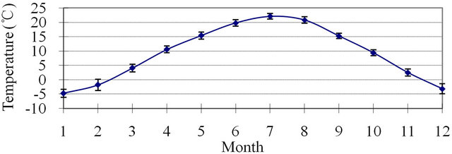 (b)
(b)
Figure 2. The monthly mean precipitation (a) and monthly mean air temperature (b) averaged during the years 1957- 2001 at the experimental site (vertical bars show standard deviations).
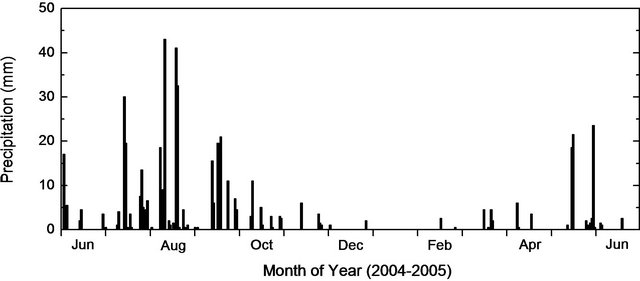
Figure 3. Daily precipitation during June 2004 to June 2005.
not much. During the remaining days of July, through August, and until the end of September, rainfall events occurred very frequently, many of which had quite prominent precipitation. The maximum precipitation occurred on August 11 and August 19, with the daily values of 42 mm and 41 mm respectively. The accumulated precipitation during the period of July 9 to September 30 was 339 mm, whereas that during June 1 to July 8 was only 36 mm. Therefore, we will use the duration of June and the first week of July to represent the dry season over the studied region, and from the second week of July until the end of September to represent the wet season. We will focus on analyzing fluxes properties during these dry and wet seasons.
3. Instrumentation
In this experiment, a flux and radiation observation system (FROS) was installed to measure turbulent fluxes and radiation components in the atmospheric surface layer. The FROS included three ultrasonic anemometer/thermometers (1210R3; GILL Instruments, Ltd., UK) mounted at 2 m, 12 m, and 32 m heights measuring turbulent quantities of wind and air temperature, as well as three open-path infrared CO2/H2O gas analyzers (LI-7500; Li-Cor, Inc., USA) recording the fluctuations of CO2 and water vapor densities at the three heights. Two shortwave radiometers (CM21; Kipp & Zonen B.V., Netherlands) and two longwave radiometers (CG4; Kipp & Zonen B.V., Netherlands) were installed at 2 m level to measure the upward/downward shortwave radiations and upward/downward longwave radiations. Soil thermometers (CS107; Campbell Scientific Inc., USA) and soil moisture sensors (TDR-615; Campbell Scientific Inc., USA) were also used to measure the soil temperature and soil moisture at the depth of 2 cm, 10 cm, 20 cm, 40 cm, and 80 cm respectively. A rain gauge (34-T; Ohtakeiki Ltd., Japan) measured the precipitation. The data logger was the type of CR5000 by Campbell Scientific, Inc., USA.
4. Methodology
4.1. Data Selection
In this study, 10 Hz raw turbulent data measured by the ultrasonic anemometer/thermometers at three heights (2 m, 12 m, and 32 m) during the observational year (June 2004 to June 2005) were used to calculate sensible and latent heat fluxes by eddy correlation method. In section 5.1, we will focus on analyzing the properties of surface heat fluxes in the wet and dry seasons of a summer during four months (June to September in 2004) within the observational year.
Because the surface parameters CH, CE, and β are based on the assumption of surface homogeneity, to avoid the topography complexity caused by the southeast valley, these parameters were calculated only in conditions when winds came from the northwest flat terrain. In Sections 5.2 and 5.3, we will investigate the seasonal variations of bulk transfer coefficient CH for sensible heat and surface moisture availability β based on the data collected at 32 m height during the whole observational year (June 2004 to June 2005). In all these cases, we only selected clear days according to the precipitation data.
In previous studies, Matsushima and Kondo [14] described that CH was little affected by the atmospheric stability within the stability range of . Kondo and Watanabe [7] found that β was sensitive and widely dispersed when the mean wind speed was smaller than 2.0 ms−1 and the solar radiation was less than 300 Wm−2. Accordingly, we selected the data when 1) mean wind speed larger than 2.0 ms−1; 2) solar radiation larger than 300 Wm−2; 3) atmospheric stability in the range of
 .
.
4.2. Calculation of Surface Heat Fluxes and Surface Parameters
4.2.1. Surface Heat Fluxes
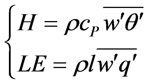
The turbulent sensible and latent heat fluxes at 2 m, 12 mand 32 m heights were calculated by the eddy covariance method, which can be formulated as following:
 (1)
(1)
Here H denotes the sensible heat flux, LE the latent heat flux; cP and ρ are the specific heat and the air density, l the latent heat for vaporization of water,  the vertical turbulent wind speed,
  the turbulent potential temperature,
 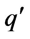 the turbulent specific humidity.
Firstly dynamic calibrations of the water vapor and CO2 densities measured by the infrared CO2/H2O gas analyzer were conducted by a standard hygrometer and standard CO2 gas [15]. The temperature measured by the ultrasonic anemometer/thermometer was calibrated by the water vapor density [16].
For flows over complex terrain, errors may arise when vector quantities are measured in a reference framework that is not consistent with that of the equations used to analyze them. To solve this problem, three mathematical rotations were applied here to transfer the sampled velocity data from the instrument’s reference frame to the streamline reference frame according to the scheme by Kaimal and Finnigan [17]. Accounting for the effect of the variation in air density due to the transport of sensible heat flux, the WPL calibration was applied in the calculation of latent heat flux [18,19].
4.2.2. Bulk Transfer Coefficients
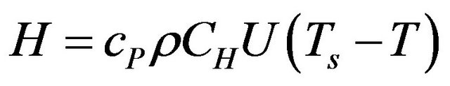
Sensible heat flux H and latent heat flux LE from a surface can be generally determined from the bulk transfer method [20]:
 (2)
(2)
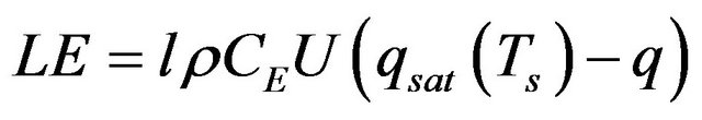 (3)
(3)
Here Ts is the surface temperature,  the saturation specific humidity at a temperature of Ts. U, T, and q represent the mean wind speed, mean air temperature, and mean specific humidity at a reference level, respectively. Here CH and CE are the bulk transfer coefficients for sensible heat and latent heat.
For a well-wetted surface,  is expected. Since the surface moisture availability β is defined as
 ,
,  for a well-wetted surface, and for a completely dry surface β = 0 can be expected; the values of β for land surfaces with different wetness vary between these limits.
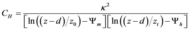
One of the methods to determine the bulk transfer coefficients is based on the Monin-Obukhov similarity theory (MOST):
 (4)
(4)
Here  and
and  are stability correction functions for momentum and heat;
 ![]() is von Kármán’s constant; z0 and zt represent the roughness length for momentum and sensible heat, respectively; and d is the displacement height [15].
is von Kármán’s constant; z0 and zt represent the roughness length for momentum and sensible heat, respectively; and d is the displacement height [15].
There are many formulations for the MOST stability functions in literatures [21-26]. In this study, we applied the interpolation stability functions for the ASL proposed by Brutsaert [26] as the following:
 (5)
(5)
 (6)
(6)
The values assigned to the constants are a = 0.33, b = 0.41, m = 1.0, c = 0.33, d = 0.057, and n = 0.78. Equations (5) and (6) can be readily integrated into
 (7)
(7)
and then yield the stability correction functions:
 (8)
(8)
 (9)
(9)
 (10)
(10)
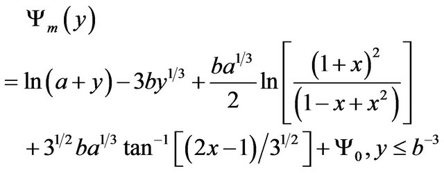
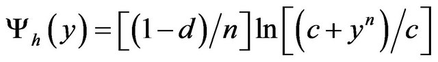
in which ,
,  , and
, and  denotes a constant of integration, given by
 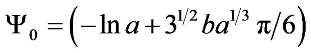 [26].
[26].
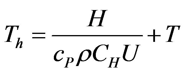
After CH is determined from (4), as an alternative, the surface temperature Ts in Equation (2) can be replaced by the effective surface temperature for sensible heat flux Th as:
 (11)
(11)
Finally from (3) the surface moisture availability β can be derived:
 (12)
(12)
After sensitivity tests, we found that the displacement height d had little effect on CH and β. Thus we applied an estimated value of d = 0.4 m and a value of z0 = 0.5 m calculated from the neutral logarithmic wind relationship based on data at 32 m height during June 2004 in determination of CH and β. To determine zt values, Sugita et al. [27] analyzed data over a complex surface and found that zt varied between 10−14 and 10−2 m. This range, together with z0 = 0.7 - 0.8 m (d = 4 m), gave a range of 4 - 32 for . Because the land cover condition in the experimental area has similar heterogeneity as that in Sugita et al. [27], we adopted a constant value of 5 to
 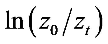 for this study and derived the corresponding value of zt.
5. Results
5.1. Surface Heat Fluxes
Before calculating surface fluxes, the flux footprint was estimated to investigate the influence of the upwind spatial distribution of the surface emission to the vertical fluxes measured at some height. The footprint was calculated by the methods given by Horst and Weil [28] and Horst [29] which allow the estimation of the upwind distance from which most of the fluxes originate for a given measurement height and atmospheric stability. We found that for our experimental site the contributed upwind distance was approximately within 2 km for the fluxes measured at 32 m level for the stability range of  .
.
5.1.1. Variations of Surface Heat Fluxes during Dry Season and Wet Season
In this section we will focus on analyzing the properties of the sensible and latent heat fluxes during the dry season (June and first week of July) and the wet season (remaining days of July, August and September in 2004) of the experimental area.
Figures 4 shows the time series of daily mean sensible and latent heat fluxes as well as net radiation from June to September in 2004. The mean sensible heat flux (denoted as H) and the mean latent heat flux (denoted as LE) showed similar fluctuation trend with the net radiation and with each other during the four months. The sensible heat flux H was close to the latent heat flux LE in June.
During July, H decreased on the whole; LE started to increase in clear days when the net radiation was also large and LE was getting larger than H gradually. The latent heat flux LE kept increasing in August and was much larger than the sensible heat flux H. The maximum of LE during August was around 200 Wm−2; in August at the study site rainfalls were concentrated and the precipitation was prominent, and most of the land surface was bare soil after the wheat was harvested in June. Thus these latent heat flux values are comparable to the results of Kimura et al. [4]. They calculated sensible and latent heat fluxes over a bare soil surface on the Loess Plateau by a three-layer soil model, and found that the latent heat flux LE in August reached a maximum of about 200 Wm−2 after a rainfall. Their modeled values of sensible heat flux H had the maximum of around 200 Wm−2 in August over the loess soil [4], which is double of our maximum H of around 100 Wm−2 during August. During September LE gradually decreased to be smaller than those in August but still showed larger than the corresponding H values.
These changes of surface heat fluxes were mainly caused by the variations of the solar radiation and the precipitation during the wet season and the dry season in the region. On one side, the decreasing of the solar radiation from June to August caused the fall of the surface temperature. In consequence, less sensible heat was available to be transferred into the atmosphere by means of turbulent processes between the land surface and the atmosphere. On the other side, the predominant increasing of the precipitation during July and August (see Figure 3) caused the surface humidity increased largely and more latent heat was produced from the land surface; similarly, the latent heat flux decreased when the precipitation during September was relatively less compared to July and August.

Figure 4. Seasonal variations in daily mean values of sensible (H) and latent (LE) heat fluxes during June to September 2004 (based on the sensors installed at 12 m height). Net radiation flux (Rn) is also drawn in the figure.
5.1.2. Detailed Analysis of Surface Fluxes
According to the different properties of sensible and latent heat fluxes during the dry and wet seasons, it should be meaningful to investigate the detailed characteristics of H and LE respectively in each season. For this purpose, we selected some typical days from both seasons with proper micrometeorological conditions such as no precipitation, clear sky in daytime, and mild wind speeds.
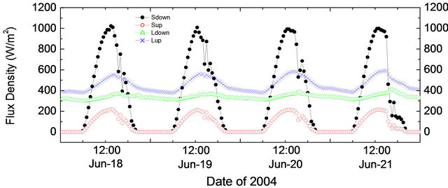
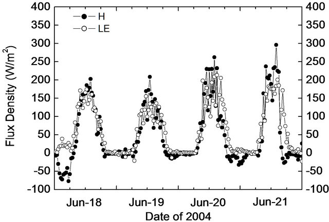
Considering the radiation components and the precipitation (see Figure 3), the four days from June 18 to 21 was selected to represent the dry season. Similarly, the duration between August 28 and 31, after strong rainfall events and with clear sky, was selected to represent the wet season.
We show the radiation components of each representative period in Figure 5. In the four representative days of dry season, the peak values of the solar radiation were around 1000 Wm−2. Their maximum of 1023 Wm−2 occurred on June 18. However in wet season, the peak values of solar radiation were about 900 Wm−2 during the four representative days, with a maximum of 952 Wm−2 on August 29, around 70 Wm−2 lower than that in the dry season.
The sensible and latent heat fluxes during both representative periods of dry and wet seasons are shown in Figure 6. In daytime of the dry period, most of the sensible heat flux H was slightly larger than the corresponding latent heat flux LE. They were generally near zero during nighttime. However, in the wet period, LE showed largely increased in daytime, much higher than H.
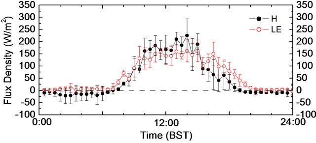
After calculating ensemble averages of H and LE during each representative period, the daily variations of H and LE are shown in Figure 7. In dry period, the maximum of H in daytime appeared at 14:00; the value was about 225 Wm−2. The peak of LE in daytime also occurred around 14:00, with a value of about 160 Wm−2. During nighttime, there was small amount of downward sensible heat flux; the values were around 25 Wm−2. After 10:00 in daytime, H tended to be larger than LE, and then kept larger until 15:30 in the afternoon. After that, H changed to be smaller than LE. At night LE was generally close to zero or was slightly minus.
In wet period, the maximum of H in daytime occurred at 11:30 with a value of 123 Wm−2. Around 15:00, H showed a second peak of 118 Wm−2. LE in daytime also showed double peak at 12:30 and 15:00, with values of 280 Wm−2 and 265 Wm−2, respectively. In nighttime, both H and LE were near to zero or slightly minus. These four representative days were shortly after the rainy days with large precipitation. Thus the surface humidity was prominently increased. Therefore, in daytime after around 10:00, strong evaporation was produced from the land surface
 (a)
(a)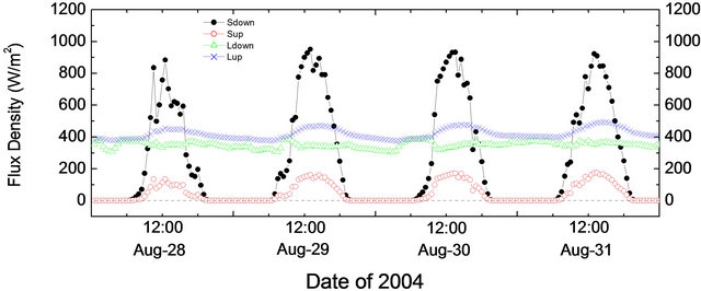 (b)
(b)
Figure 5. Time series of four radiation components during the four selected representative days in the dry period (a) and the wet period (b).
 (a)
(a)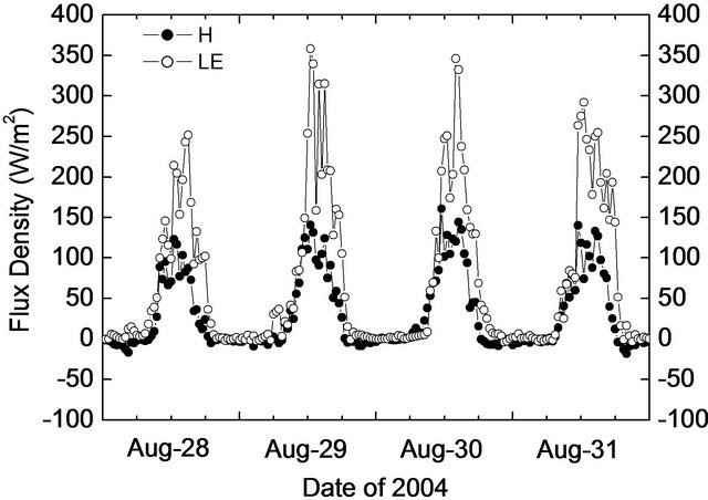 (b)
(b)
Figure 6. Time series of sensible (denoted as H) and latent (denoted as LE) heat fluxes during the four selected representative days in the dry period (a) and the wet period (b).
 (a)
(a) (b)
(b)
Figure 7. Daily variations of sensible (denoted as H) and latent (denoted as LE) heat fluxes averaged during the four selected representative days in the dry period (a) and the wet period (b).
due to heating effect by solar radiation. Such strong evaporation transferred large latent heat flux to the atmosphere, so that LE started to increase rapidly and be much higher than H. After sunset around 18:00, when the solar radiation tended to zero, LE decreased rapidly to zero.
5.2. Bulk Transfer Coefficient for Sensible Heat CH
Figure 8(a) shows the seasonal variation of the bulk transfer coefficient for sensible heat CH during June 2004 to June 2005. During the whole observational period, CH did not show very obvious change with seasons, ranging from 0.004 to 0.006; these values were higher than the values ranging between 0.002 and 0.0055 derived by Kimura and Kondo [30] over paddy fields. During June to August in 2004 and April to June in 2005, CH showed more discrete, but CH values kept more converged during October 2004 to February 2005, although still with some scattering. This can be related to the farm season in the studied area; from spring to autumn wheat and corn were planted and harvested in turn and in winter the land surface was kept bare in the farm fields. Since the wheat was usually harvested at the end of June, from the end of June in 2004, CH decreased sharply. Shimoyama et al. [31] found similar seasonal variation trends in CH and surface roughness length from a Siberian bog, and indicated that change in CH depended on the physical effects of surface roughness so that canopy structure had effect on seasonal variation of CH. Kimura and Kondo [30] also observed that CH changed with the height of canopy in paddy fields.
5.3. Surface Moisture Availability β
Figure 8(b) shows the seasonal variation of the surface moisture availability β from June 2004 to June 2005. During these 13 months, the values of β changed obviously with seasons. Higher values were typically found in June and July 2004, with large scattering; the peak value was 0.91 occurring on July 17. From October 2004, β gradually decreased, and reached the lowest value around 0.03 in February 2005. After that, β was increasing from the middle of April until the end of June in 2005. The mean value of β during the wet season of the region was 0.29; this value was much lower than the values between 0.5 - 0.8 over a paddy field derived by Kimura and Kondo [30] and higher than the values within 0.1 - 0.2 over a forest by Kondo [32]. The mean β value was 0.19 in winter; this value was comparable with the values between 0.1 - 0.2 from the forest [32] with the close roughness length of 0.3 - 1 m to that in this study. Because a higher CH value will cause a lower β value, this forest also showed a comparable CH value of 0.005
 (a)
(a)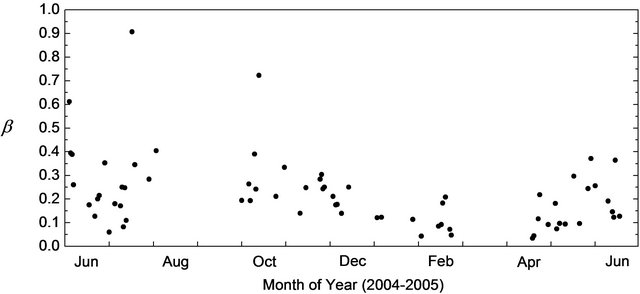 (b)
(b)
Figure 8. Seasonal variations of (a) the bulk transfer coefficient for sensible heat CH and (b) the surface moisture availability β on the plateau during June 2004 to June 2005. Both values were evaluated only when the wind direction was from north-west (over the flat terrain).
with the CH values in this study [32]. Kimura and Kondo [30] calculated β over a rice paddy field; and their β values decreased to around 0.7 after the irrigation periods.
Figure 9 shows the relationship between the surface moisture availability β and the soil water content measured at 10 cm depth at the experimental site. In this plot, β values show clear dependence on the surface soil water content; the three highest values of β correspond to high soil water content which were observed on the days after the raining days with large daily precipitation. These indicate the importance of soil water content in determining β; the soil water content change contributes much to the variations of surface moisture availability.
6. Conclusions and Discussions
The energy fluxes and surface parameters over acomplex surface on the Loess Plateau were investigated in this study. For the flux measurement, the upwind distance of 70% flux contribution was approximately 2 km in the atmospheric stability range of neutral to weakly unstable. The dry season in the observational region occurred from

Figure 9. Relationship between the surface moisture availability and the soil water content measured at 10 cm depth (regression line: Y = 0.04344 + 1.22788X; r2 = 0.27).
June to the first week of July in 2004; from the middle of July the region got into the wet season until the end of September in 2004.
In dry season the surface transferred turbulent energy to the ABL mainly by means of sensible heat flux with a maximum of around 230 Wm−2. During the wet season, latent heat flux increased prominently reaching a peak around 280 Wm−2 and sensible heat flux decreased having a maximum half of that in dry season; the land surface mainly offered latent heat into the atmospheric surface layer.
The bulk transfer coefficient for sensible heat CH did not change obviously with seasons and had the values between 0.004 and 0.006 during the observational year. The surface moisture availability β changed with seasons with higher values in June and July 2004 and lowest values around 0.03 in February 2005. Its peak value of 0.91 occurred on July 17 in 2004. During the wet season the mean value of β was 0.29. In the winter the mean value of β was 0.19, which was comparable with the values from a forest [32] which had a comparable roughness length as this study. The surface soil water content showed related to β; the highest values of β corresponded to the highest soil water content.
Because of the intricate topography on the Loess Plateau and the heterogeneity of the surface coverage in the experimental area, in this paper we only chose winds from the flat terrain direction to analyze the bulk heat transfer properties, more work will be meaningful to investigate the regional heat transfer and energy balance on the plateau based on synergistic approaches including remote sensing and numerical modeling.
7. Acknowledgements
This study was part of the research project of Recent Rapid Change of Water Circulation in the Yellow River and its Effects on the Environment supported by the Research Institute for Humanity and Nature, Japan. We thank all the members in our experimental team and other cooperative staffs in the Institute of Soil and Water Conservation, Chinese Academy of Sciences. We also give our special thanks to Dr. Sukanta Basu for his comments on revising this paper.
REFERENCES
- J. C. Wyngaard, “Scalar Fluxes in the Planetary Boundary Layer—Theory, Modeling, and Measurement,” Boundary-Layer Meteorology, Vol. 50, No. 1-4, 1990, pp. 49- 75. doi:10.1007/BF00120518
- T. Hiyama, A. Takahashi, A. Higuchi, M. Nishikawa, W. Li, W. Liu and Y. Fukushima, “Atmospheric Boundary Layer Observations on the Changwu Agro-Ecological Experimental Station over the Loess Plateau, China,” Asia Flux Newsletter, No. 16, 2005, pp. 5-9.
- R. Kimura, N. Takayama, M. Kamichika and N. Matsuoka, “Soil Water Content and Heat Balance in the Loess Plateau—Determination of Parameters in the Three-Layered Soil Model and Experimental Result of Model Calculation,” Journal of Agricultural Meteorology, Vol. 60, No. 1, 2004, pp. 55-65. doi:10.2480/agrmet.60.55
- R. Kimura, M. Kamichika, N. Takayama, N. Matsuoka and X. C. Zhang, “Heat Balance and Soil Moisture in the Loess Plateau, China,” Journal of Agricultural Meteorology, Vol. 60, No. 2, 2004, pp. 103-113. doi:10.2480/agrmet.60.103
- S. Liu, R. Sun, Z. Sun, X. Li and C. Liu, “Evaluation of Three Complementary Relationship Approaches for Evapotranspiration over the Yellow River Basin,” Hydrological Processes, Vol. 20, No. 11, 2006, pp. 2347-2361. doi:10.1002/hyp.6048
- I. Tamagawa, “Turbulent Characteristics and Bulk Transfer Coefficients over the Desert in the HEIFE Area,” Boundary-Layer Meteorology, Vol. 77, No. 1, 1996, pp. 1-20. doi:10.1007/BF00121856
- J. Kondo and T. Watanabe, “Studies on the Bulk Transfer Coefficients over a Vegetated Surface with a Multilayer Energy Budget Model,” Journal of the Atmospheric Sciences, Vol. 49, No. 23, 1992, pp. 2183-2199. doi:10.1175/1520-0469(1992)049<2183:SOTBTC>2.0.CO;2
- H. K. Kafle and Y. Yamaguchi, “Effects of Topography on the Spatial Distribution of Evapotranspiration over a Complex Terrain Using Two-Source Energy Balance Model with ASTER Data,” Hydrological Processes, Vol. 23, No. 16, 2009, pp. 2295-2306. doi:10.1002/hyp.7336
- W. P. Kustas, F. Li, T. J. Jackson, J. H. Prueger, J. I. MacPherson and M. Wolde, “Effects of Remote Sensing Pixel Resolution on Modeled Energy Flux Variability of Croplands in Iowa,” Remote Sensing of Environment, Vol. 92, No. 4, 2004, pp. 535-547. doi:10.1016/j.rse.2004.02.020
- W. Li, T. Hiyama and N. Kobayashi, “Turbulence Spectra in the Near-Neutral Surface Layer over the Loess Plateau in China,” Boundary-Layer Meteorology, Vol. 124, No. 3, 2007, pp. 449-463. doi:10.1007/s10546-007-9180-y
- M. Nishikawa,T. Hiyama, K. Tsuboki and Y. Fukushima, “Numerical Simulations of Local Circulation and Cumulus Generation over theLoess Plateau, China,” Journal of Applied Meteorologyand Climatology, Vol. 48, No. 4, 2009, pp. 849-862. doi:10.1175/2008JAMC2041.1
- A. Takahashi, T. Hiyama, M. Nishikawa, H. Fujinami, A. Higuchi, W. Li, W. Liu and Y. Fukushima, “Diurnal Variation of ater Vapor Mixing between the Atmospheric Boundary Layer and Free Atmosphere over Changwu, the Loess Plateau in China,” SOLA, Vol. 4, 2008, pp. 33-36. doi:10.2151/sola.2008-009
- N. Takayama, R. Kimura, M. Kamichika, N. Matsuoka and X. C. Zhang, “Climatic Features of Rainfall in the Loess Plateau in China,” Journal of Agricultural Meteorology, Vol. 60, No. 3, 2004, pp. 173-189. doi:10.2480/agrmet.60.173
- D. Matsushima and J. Kondo, “A Proper Method for Estimating Sensible Heat Flux above a Horizontal-Homogeneous Vegetation Canopy Using Radiometric Surface Observations,” Journal of Applied Meteorology, Vol. 36, No. 12, 1997, pp. 1696-1711. doi:10.1175/1520-0450(1997)036<1696:APMFES>2.0.CO;2
- K. Shimoyama, T. Hiyama, Y. Fukushima and G. Inoue, “Seasonal and Inter Annual Variation in Water Vapor and Heat Fluxes in a West Siberian Continental Bog,” Journal of Geophysical Research, Vol. 108, No. D20, 2003, p. 4648. doi:10.1029/2003JD003485
- J. C. Kaimal and J. E. Gaynor, “Another Look at Sonic Thermometry,” Boundary-Layer Meteorology, Vol. 56, No. 4, 1991, pp. 401-410. doi:10.1007/BF00119215
- J. C. Kaimal and J. J. Finnigan, “Atmospheric Boundary Layer Flows,” Oxford University Press, New York, 1994.
- E. K. Webb, G. I. Pearman and R. Leuning, “Correction of Flux Measurements for Density Effects Due to Heat and Water Vapour Transfer,” Quarterly Journal of the Royal Meteorological Society, Vol. 106, No. 447, 1980, pp. 85-100. doi:10.1002/qj.49710644707
- R. Leuning and J. Moncrieff, “Eddy-Covariance CO2 Flux Measurements using Openand Closed-Path CO2 Analyzers: Corrections for Analyzer Water Vapor Sensitivity and Damping of Fluctuations in Air Sampling Tubes,” Boundary-Layer Meteorology, Vol. 53, No. 1-2, 1990, pp. 63-76. doi:10.1007/BF00122463
- W. Brutsaert, “Evaporation into the Atmosphere: Theory, History, and Applications,” Kluwer Academic Publishers, Boston, 1982.
- J. C. Wyngaard and O. R. Cote, “The Budgets of Turbulent Kinetic Energy and Temperature Variance in the Atmospheric Surface Layer,” Journal of Atmospheric Sciences, Vol. 28, No. 2, 1971, pp. 190-201. doi:10.1175/1520-0469(1971)028<0190:TBOTKE>2.0.CO;2
- J. C. Wyngaard, “On Surface-Layer Turbulence,” In: D. A. Haugen, Ed., Workshop on Micrometeorology, American Meteorological Society, Boston, 1973, pp. 101-149.
- E. L. Andreas, “Two-Wavelength Method of Measuring Path-Averaged Turbulent Surface Heat Fluxes,” Journal of Atmospheric and Oceanic Technology, Vol. 6, No. 2, 1989, pp. 280-292. doi:10.1175/1520-0426(1989)006<0280:TWMOMP>2.0.CO;2
- R. J. Hill, “Review of Optical Scintillation Methods of Measuring the Refraction-Index Spectrum, Inner Scale and the Surface Fluxes,” Wave Random Media, Vol. 2, No. 3, 1992, pp. 179-201. doi:10.1088/0959-7174/2/3/001
- W. Brutsaert, “Stability Correction Functions for the Mean Wind Speed and Temperature in the Unstable Surface Layer,” Geophysical Research Letters, Vol. 19, No. 5, 1992, pp. 469-472. doi:10.1029/92GL00084
- W. Brutsaert, “Aspects of Bulk Atmospheric Boundary Layer Similarity under Free-Convective Conditions,” Reviews of Geophysics, Vol. 37, No. 4, 1999, pp. 439-451. doi:10.1029/1999RG900013
- M. Sugita, T. Hiyama and I. Kayane, “How Regional are the Regional Fluxes Obtained from Lower Atmospheric Boundary Layer Data?” Water Resources Research, Vol. 33, No. 6, 1997, pp. 1437-1445. doi:10.1029/97WR00569
- T. W. Horst and J. C. Weil, “How Far is Far Enough— The Fetch Requirements for Micrometeorological Measurement of Surface Fluxes,” Journal of Atmospheric and Oceanic Technology, Vol. 11, No. 4, 1994, pp. 1018- 1025. doi:10.1175/1520-0426(1994)011<1018:HFIFET>2.0.CO;2
- T. W. Horst, “The Footprint for Estimation of Atmosphere-Surface Exchange Fluxes by Profile Techniques,” Boundary-Layer Meteorology, Vol. 90, No. 2, 1999, pp. 171-188. doi:10.1023/A:1001774726067
- R. Kimura and J. Kondo, “Heat Balance Model over a Vegetated Area and Its Application to Paddy Field,” Journal of the Meteorological Society of Japan, Vol. 76, No. 2, 1998, pp. 937-953.
- K. Shimoyama, T. Hiyama, Y. Fukushima and G. Inoue, “Controls on Evapotranspiration in a West Siberian Bog,” Journal of Geophysical Research, Vol. 109, No. D8, 2004, Article ID: D08111. doi:10.1029/2003JD004114
- J. Kondo, “Meteorology of the Water Environment: Water and Heat Balance of the Earth’s Surface,” Asakura Shoten Press, Tokyo, 1994.