Journal of Signal and Information Processing
Vol.4 No.2(2013), Article ID:31059,3 pages DOI:10.4236/jsip.2013.42024
Maximal Phase Space Compression*
![]()
Institute for Physics and Nuclear Engineering, Bucharest, Romania.
Email: modima@nipne.ro
Copyright © 2013 Mihai Dima, Marian Petre. This is an open access article distributed under the Creative Commons Attribution License, which permits unrestricted use, distribution, and reproduction in any medium, provided the original work is properly cited.
Received December 29th, 2012; revised January 31st, 2013; accepted February 10th, 2013
Keywords: Quantum Compression
ABSTRACT
The (seldomly quoted) generalised-Heisenberg uncertainty relations are an effect of the quantum correlation coefficient inequalities. The quantum correlation coefficient determines how much a state can be compacted and on what basis. It is shown that how this can be used to best compress a signal (such as a radio wave, or a 2D laser complex field at a focal plane) while at the same time encrypting the signal.
1. Introduction
The concept of correlation coefficient originates in statistics where one quantity, say k, is approximately correlated to another, say x, plus some random noise.
The degree of correlation [1-4] (or noise absence) is expressed by the quantity a in the interval  defined as:
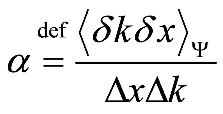
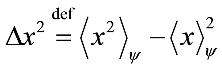
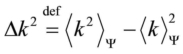
where:
In quantum mechanics the above definition is retained, the averages being replaced with averages over the state in causa. The number in this case is complex, with both real and imaginary parts in the interval , and the norm less than unity.
The real-part of the quantum correlation coefficient is:
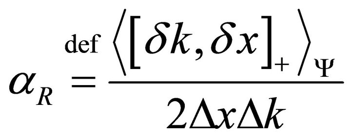
Since x and k are self-adjoint, it is evident that  will be self-adjoint, hence have real valued averages.
The imaginary-part of the quantum correlation coefficient is:
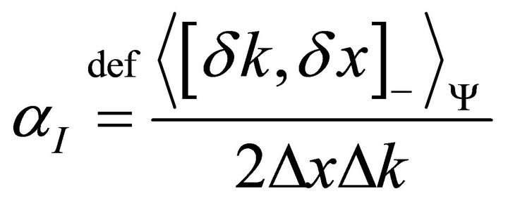
Again, since x and k are self-adjoint operators, it is evident that  will be anti-adjoint. This implies that its average
  will have imaginary values.
For canonically conjugate observables  , aI depends only on the inverse of the state’s spread in x and k space.
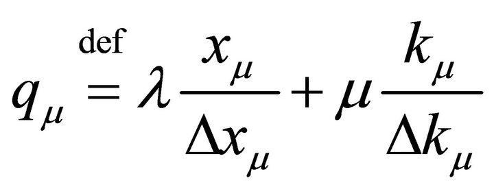
A mixed x-k operator can be defined as:

The operator is not necessarily self-adjoint, however it is evident that:
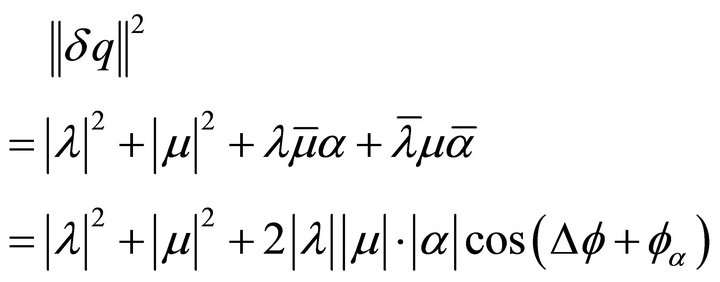
This can be further written as:
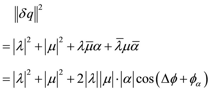
where  is the phase difference between l and m and fa the phase of a.
From  it follows now that:
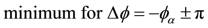
which is valid for any phase combination Dj, therefore,
in turn valid for all l and m, hence,
which is to say,  , in good analogy to its statistical counterpart.
2. Generalized Heisenberg Relations
However, in the quantum case, there is more than just one inequality, due to:
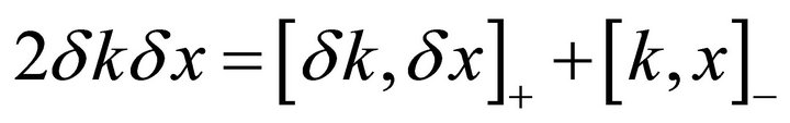
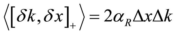
for self-adjoint operators the second term being antiadjoint, while the first self-adjoint:
For canonically-conjugate variables the second term is (up to a sign convention):
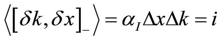
hence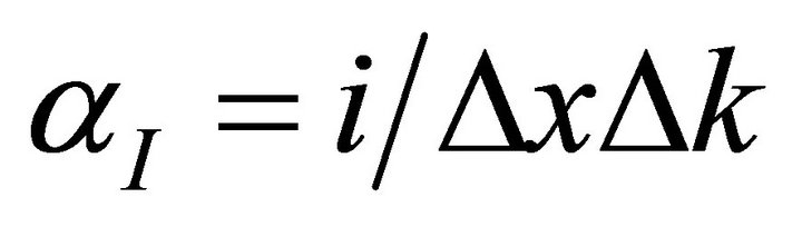 .
.
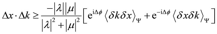
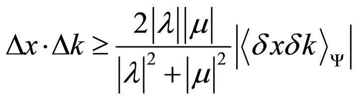
Using:  the above two can be used to express
 :
:
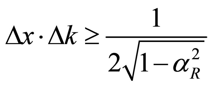
which is the generalized Heisenberg inequality [5-10]. This relation shows that, for states with a high real-part correlation coefficient, the product of the two uncertainties can actually be very large, and the minimum value of  is quite remote.
3. Signal Compression
Such a situation is ideal for signal compression since any wave (RF signal in 1D, or laser field at a focal plane, in 2D) can be viewed as a state.
Consider again the q-operator:
The idea is that, for instance, a spike in real space is very concentrated, while in Fourier space it extends to infinity uniformly. Conversely, a wave is very concentrated in Fourier space, but extended to infinity in realspace (the Heisenberg uncertainty relations above).
Does there exist an “intermediate”, rotated-space between the realand Fourier-spaces, in which an arbitrary signal is best compressed [11]?
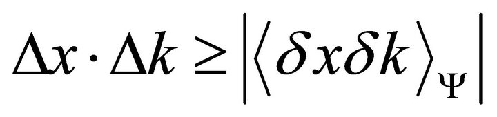
It would be of interest, in this respect, that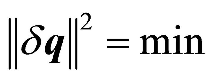 , or
, or
 :
: ..
..
From here further, the minimum is achieved by reference to some volumic (or scaling) condition, symmetrical in  and
and :
:
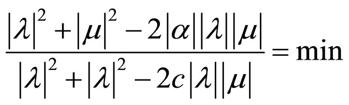
where:
1)  would be an ad-hoc canonical norm;
2)  would be a comparison to classical (statistical) compression, etc. The above condition reaches extremae for:
1)  the fraction would just be constant;
2)  would be again a constant fraction;
3)  with minimum for the two equal.
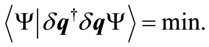
Solution (3) is independent of the choice for c, yielding the best operator to use:
in its eigen-value spanned space, the signal occupying minimum volume:
An example of perfectly quantum-correlated,  , quantities are the spin operator components sx and sy in a sz state-depending on the
  case, the q operator being in this case s±.
4. q-Eigen Vectors and Values
Firstly note that q† ¹ q implies complex eigen-values. From the eigen-value equation  the eigen-vectors are:
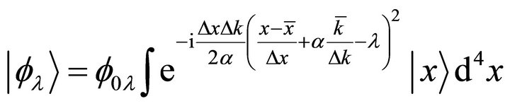
where  is such that the state norms to unity. For such (Gaussian) states
 . It follows directly that
 . Since
 , its average is real and therefore the complex part of λ is proportional to its real part:
 .
.
Thus the eigen-values are constrained to a line passing through zero in the complex plane, possible to describe with just one real parameter.
A Fourier [12,13] analysis can be now performed on  with the eigen-vectors
  yielding a more compact spectrum than the traditional Fourier spectrum:
On reconstruction the signal  is found as:
where . Due to the latter, for signal processing, this is similar to traditional Fourier analysis [12, 13].
5. Signal Compression
Both classical and quantum signals contain information that behaves “quantum” in nature. Examples thereof would be a 2D laser field at its focal plane, for the quantum, and an RF signal (in 1D), for the classical. In both cases the “quantum” nature is evidentiated by the (complex) quantum correlation coefficient α. This coefficient allows the design of a “rotated” Fourier transform (between real space and Fourier space) in which the signal is best compacted.
Said compactification brings also non-statistical encryption of the signal, rendering obsolete traditional codebreaking methods [5-10].
REFERENCES
- R. Bracewell, “The Autocorrelation Function. The Fourier Transform and Its Applications,” McGraw-Hill, New York, 1965.
- W. H. Press, B. P. Flannery, S. A. Teukolsky and W. T. Vetterling, “Correlation and Autocorrelation Using the FFT,” In: W. H. Press, S. A. Teukolsky, W. T. Vetterling and B. P. Flannery, Eds., Numerical Recipes in FORTRAN: The Art of Scientific Computing, 2nd Edition, Cambridge University Press, Cambridge, 1992, p. 538.
- R. Bracewell, “The Fourier Transform and Its Applications,” 3rd Edition, McGraw-Hill, New York, 1999.
- G. B. Folland, “Real Analysis: Modern Techniques and their Applications,” 2nd Edition, Wiley, New York, 1999.
- E. Schrödinger, “On the Heisenberg(ian) Uncertainty Principle,” Berl. Ber., Vol. 19, 1930, p. 296.
- E. Schrödinger, “Collected Papers Vol. 3: Contributions to Quantum Theory,” Austrian Academy of Sciences, Vienna, 1984, p. 348.
- D. Bohm, “Quantum Theory,” Prentice Hall, Upper Saddle River, 1951, p. 199.
- E. Merzbacher, “Quantum Mechanics,” 2nd Edition, Wiley, New York, 1970, p. 158.
- J. M. Lévy-Leblond, “Correlation of Quantum Properties and the Generalized Heisenberg Inequality,” American Journal of Physics, Vol. 54, No. 2, 1986, p. 135.
- L. Goldenberg and L. Vaidman, “Applications of a Simple Quantum Mechanical Formula,” American Journal of Physics, Vol. 64, No. 8, 1996, p. 1059.
- R. W. Henry and S. C. Glotzer, “A squeezed State Primer,” American Journal of Physics, Vol. 56, 1988, p. 318.
- G. Arfken, “Development of the Fourier Integral, Fourier Transforms—Inversion Theorem, and Fourier Transform of Derivatives,” In: Mathematical Methods for Physicists, 3rd Edition, Academic Press, Orlando, 1985, p. 794.
- J. F. James, “A Student’s Guide to Fourier Transforms with Applications in Physics and Engineering,” Cambridge University Press, New York, 1995.
NOTES
*One of us (M. Petre) acknowledges support under a grant of the Romanian National Authority for Scientific Research, CNCS-UEFISCDI, project number PN-II-ID-PCE-2011-3-0323; one of us (M. Dima) acknowledges support under ANCS Grant PN09370104.