Journal of Applied Mathematics and Physics
Vol.04 No.08(2016), Article ID:70200,30 pages
10.4236/jamp.2016.48175
Modeling and Simulation of Real Gas Flow in a Pipeline
Agegnehu Atena, Tilahun Muche
Department of Mathematics, Savannah State University, Savannah, USA

Copyright © 2016 by authors and Scientific Research Publishing Inc.
This work is licensed under the Creative Commons Attribution International License (CC BY).
http://creativecommons.org/licenses/by/4.0/


Received 21 July 2016; accepted 27 August 2016; published 30 August 2016
ABSTRACT
In this paper, a mathematical model that describes the flow of gas in a pipe is formulated. The model is simplified by making some assumptions. It is considered that the natural gas flowing in a long horizontal pipe, no heat source occurs inside the volume, transfer of heat due to heat conduction is dominated by heat exchange with the surrounding. The flow equations are coupled with equation of state. Different types of equations of state, ranging from the simple Ideal gas law to the more complex equation of state Benedict Webb Rubin Starling (BWRS), are considered. The flow equations are solved numerically using the Godunov scheme with Roe solver. Some numerical results are also presented.
Keywords:
Gas Flow, Equation of State, Godunov Scheme, Roe Solver, Pipe

1. Introduction
The purpose of this paper is to describe the flow of natural gas in a pipeline by employing the full set of differential equations along with different types of equations of states(EOS), ranging from the simple Ideal gas law to the more complex equation of state, Benedict Webb Rubin Starling (BWRS). The flow equations are derived from the physical principles of conservation of mass, momentum, and energy. More detailed discussion of conservation laws can be found in [1] - [4] . The natural gas is inviscid and compressible. The gas flows in along a horizontal pipe, and then can be considered as one-dimensional flow. It is assumed no heat source occurs inside the pipe and transfer of heat due to the heat conduction is much less than the heat exchange with the surrounding.
In this paper, the results obtained by solving the flow equations along with different types of EOS are compared [5] . The ideal gas equation works reasonably well over limited temperature and pressure ranges for many substances. However, pipelines commonly operate outside these ranges and may move substances that are not ideal under any conditions. The more complicated EOS will approximate the real gas behavior for a wide range of pressure and temperature conditions.
The Godunov scheme with Roe solver [3] is used to solve the Euler equations numerically. The Godunov scheme for conservation laws is known for its shock-capturing capability.
The rest of the article is organized as follows. In Section (2) we review the set of partial differential equations which describe the flow of gas in a pipe. Several equations of states are discussed in this section. In Section (3) a thermodynamical relationships among the physical quantities are presented. One can refer [6] for more thermodynamical relationships. Section (4) contains the discussion of the numerical method used to solve the flow equations together with different types equation of states. Some numerical results are given in this section. Conclusions are deferred to Section (5).
2. Governing Equations of Real Gas Flow in a Pipe
Let us consider a gas occupying a sub domain  at time
 . Let
. Let  describes the position of the particle
  at time t. Then at time t the gas occupies the domain
 . The velocity of the gas at position x and time t is given by
 .
.
2.1. Transport Theorem
Let  be some physical quantity transported by the fluid. The total amount
  of the quantity f contained in
  a time t is given by
 .
.
Notation: 
The rate of change of  is given by:
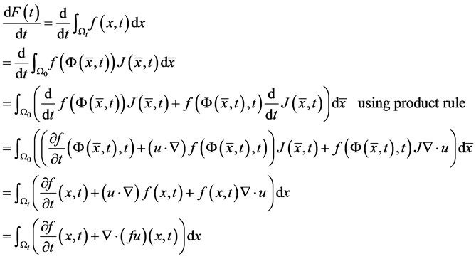
Then we get the transport theorem: . The transport theorem
is useful in the derivation of the governing equations.
2.2. Conservation of Mass (The Continuity Equation)
The total mass m in a volume  is given by
 . Mass is conserved during the deformation of
 i.e.
i.e. ,
, 
 (By transport theorem)
 (1)
(1)
Since the above integral holds true for arbitrary region 
2.3. Conservation of Momentum (Equation of the Motion)
The total momentum M of particles contained in  is given by
According to Newton’s second law: The rate of change of momentum equals the action of all the forces F applied on 


We have two types of forces acting on :
:
1) Volume forces , for example gravitation, which is given by

where g is the gravitational acceleration.
2) Surface forces  acting on
  through the boundary
  of
of , such as pressure and inner friction forces.
Surface forces are given by

where  is the stress tensor defined as:

and  is the outer normal. The total force
 . Then, we have
 .
.
By applying divergence theorem, the second term on the right side of the above equation can be transformed to integral over the domain  and then we get:

 or
or

For Newtonian fluid, the stress tensor depends linearly on the deformation velocity,  , i.e.

where  is the viscous part of
 , p is pressure, I is the identity matrix,
  and
and  are friction coefficients, and D is the strain tensor given by

For inviscid fluid, friction is neglected and then 
Therefore, the equation of motion for inviscid fluid becomes
 (2)
(2)
2.4. Conservation of Energy
Conservation of energy accounts for effects of temperature variations on the flow or the transfer of heat with in the flow. The 1st Law of Thermodynamics states that: The total energy of a system and its surroundings remains constant.
Let  be the total energy of the fluid in
  and Q be the amount of heat transfered to
 . The rate of change of the total energy of the fluid occupying
  is the sum of powers of the volume force acting on the volume
 , powers of the surface force acting on the surface
 , and the amount of heat transmitted to
 , i.e.

where  and
and  is the density of energy (per unit mass), e is internal energy
density, and  is the density of kinetic energy.

where q is the density of heat sources (per unit mass), and
 is the heat flux (transfer of heat by conduction).
The transfer of heat by conduction is given by Fourier’s law:
 where T is the absolute temperature and
  is the coefficient of thermal conductivity of the fluid.
 is the density of heat transfered from the surrounding and is given by:
 where
where  is the total heat transfer coefficient and
  is the temperature of the surrounding.
Then the energy equation for inviscid gas flow becomes:

By applying the transport and divergence theorems to the above equation we obtain the following equation:


 .
.
 (3)
(3)
There fore, from the equations (1), (2), (3) we get the following system of equations.
 (4)
(4)
2.5. Simplifications
In practice the form of mathematical model varies with the assumptions made as regards of operation conditions of the pipeline. Simplified models are obtained by neglecting some terms in the basic equations. In our case, we consider natural gas (Methane) flowing in a long horizontal pipeline. Hence we can consider the flow as a one dimensional flow. By assuming the pipe is horizontal, we can neglect the contribution of the gravitational force.
Assume also no heat source occurs inside the volume. For a cylindrical pipe,  where D is the
diameter of the pipe. By applying the assumptions we made, (4) is reduced to
 (5)
(5)
Furthermore, Methane gas has the following properties. The specific heat capacity , thermal conductivity
 , dynamic viscosity
 . Typical values for the overall heat transfer coefficient
  are
are  for 0.5 m diameter insulated and buried in soil. If the pipe is exposed on the air
  is
is .
.
Prandtl number (Pr), defined as , describes the relative strength of viscosity (the diffusion of
momentum) to that of heat. It is entirely a property of the fluid not the flow. In our case the value of Pr is about 0.7, this enables us to regard the flow as inviscid flow. For gas flow typical values of Pr are between 0.7 and 1. Another dimensionless constant we can use to simplify our system of equations is the Nusselt number (Nu). The
Nusselt number is defined as , where D is a characteristic width of a flow, for example the diameter
of the pipe. The Nusselt number compares convection heat transfer to fluid conduction heat transfer.
For Methane gas flowing through an insulated pipe of diameter 0.5 m buried underground, the value of Nu is approximately 10. If the pipe is exposed to air, it will be around 300. Therefore, the term included in the energy
equation due to heat conduction  can be neglected in favor of the term due to heat exchange with the surrounding
 . Incorporating these assumptions to Equation (5) yields:
 (6)
(6)
where  is an equation of state used to complete the system of conservation laws. In the next chapter we will solve Equation (6) with different equation of state numerically.
2.6. Equation of State (EOS)
An equation of state is a relationship between state variables, such that specification of two state variables permits the calculation of the other state variables. For an ideal gas, the equation of state is the ideal gas law. More complicated EOS have been formulated by several workers to try to model the behavior of real gases over a range of pressures and temperatures. This includes Van der Waals (VDW), Sovae Redlich Kwong (SRK), Peng Robinson (PR), and Benedict Webb Rubin Starling (BWRS).
2.6.1. Ideal Gas law
The ideal gas law is given by
 (7)
(7)
where p is the pressure,  is the density, R is the gas constant, and T is the absolute temperature.
The ideal gas law is derived based on two assumptions:
The gas molecules occupy a negligible fraction of the total volume of the gas.
The force of attraction between gas molecules is zero.
The ideal gas equation works reasonably well over limited temperature and pressure ranges for many substances. However, pipelines commonly operate outside these ranges and may move substances that are not ideal under any conditions. Hence, we need to look for equation of state with wider validity.
2.6.2. Van der Waals (VDW) EOS
It was observed that the ideal gas law didn’t quite work for higher pressures and temperatures. The first assumption works at low pressures. But this assumption is not valid as the gas is compressed. Imagine for the moment that the molecules in a gas were all clustered in one corner of a cylinder, as shown in the figure below. At normal pressures, the volume occupied by these particles is a negligibly small fraction of the total volume of the gas. But at high pressures (when the gas is compressed), this is no longer true. As a result, real gases are not as compressible at high pressures as an ideal gas. The volume of real gas is therefore larger than expected from the ideal gas equation at high pressures. Van der Waals proposed that we correct for the fact that the volume of real gas is too large at high pressures by subtracting a term from the volume of the real gas before we substitute it in to the ideal gas equation. He therefore introduced a constant b in to the ideal gas equation that was equal to the volume actually occupied by the gas particles. When the pressure is small, and the volume is reasonably large, the subtracted term is too small to make any difference in the calculation. But at high pressures, when the volume of the gas is small, the subtracted term corrects for the fact that the volume of a real gas is larger than expected from the ideal gas equation.
The assumption that there is no force of attraction between the gas particles cannot be true. If it was, gases would never condense to form liquids. In reality, there is a small force of attraction between gas molecules that tends to hold the molecules together. This force of attraction has two consequences: (1) gases condense to form liquids at low temperatures and (2) the pressure of a real gas is sometimes smaller than expected for an ideal gas. To correct for the fact that the pressure of a real gas is smaller than expected from the ideal gas equation, Van der Waals added a term to the pressure in the ideal gas equation. This term contains a second constant a. The complete Van der Waals equation is written as follows:
 (8)
(8)
Or in terms of molar volume

where


R is gas constant,  critical pressure, and
  critical temperature Note that the values of the constants a and b differ from gas to gas. Even though, VDW EOS is better than Ideal gas law, still it is inadequate to describe real gas behavior.
We will consider three widely used equations of state that do work reasonably well near the dew point: Sovae-Redlich-Kwong (SRK), Peng-Robinson (PR), and Benedict-Webb-Rubin-Starling (BWRS). In addition to covering a wide range of conditions, these equations also can be expressed in generalized forms with mixing rules that permit the calculation of the coefficients for different compositions.
SRK and PR, along with VDW are called cubic equation of state, because expansion of the equations into a polynomial results in the highest order terms in density (or specific volume) being cubic. BWRS adds fifth and sixth power and exponential density terms. The cubic equation are all of the form
 (9)
(9)
2.6.3. The Sovae-Redlich-Kwong (SRK) EOS
The SRK EOS of state is given by
 (10)
(10)
where


w is the accentric factor which is a measure of the gas molecules deviation from the spherical symmetry, R is
gas constant,  critical pressure,
  critical temperature, and
  is the reduced temperature.
2.6.4. The Peng-Robinson (PR) EOS
The PR EOS is defined as
 (11)
(11)
where


2.6.5. Benedict-Webb-Rubin-Starling (BWRS) EOS
Probably because of its ability to cover both liquids and gases and the availability of coefficients and mixing rules for many hydrocarbons in one place, BWRS is the most widely used equation of state for simulation of pipelines with high density hydrocarbons, or with condensation.
Simplicity is not among the good qualities of the BWRS equation of state. The form of the equation is:
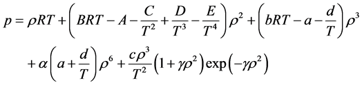 (12)
(12)
where the eleven coefficients , and
, and  are determined from
  and
and  of the gas of interest and the universal constants
  and
and  as follows.


where


BWRS can be adapted for mixtures by the rules:


where  is the mole fraction of the pure component i of the mixture, and
  are the binary interaction coefficients.
2.6.6. The Universal Gas Law
The universal gas law is  where Z is called the compressibility factor (Real gas factor). It is a measure of how far the gas is from ideality. At atmospheric conditions, the value of Z is typically around 0.99. Under pipeline conditions, the value is typically around 0.9. A good equation of state can be selected by its ability to approximate the compressibility factor at critical conditions
 .
.
For example the experimental value of  for Methane is 0.288. But its approximate value by VDW is 0.3025, by SRK is 0.2904, by PR it is 0.2894, and by BWRS it is 0.2890.
3. Thermodynamical Relations
In this section we will briefly discuss thermodynamical relations that exist among different physical quantities. First law of thermodynamics states that
 (13)
(13)
The specific total enthalpy is defined as  which implies
 (14)
(14)
Derivative relationships:
Assume , then
 . Comparing the coefficients of this equation to that of Equation (13) we get
 (15)
(15)
Similarly, assuming  we get

And comparing the coefficient of this equation with that of Equation (14) we get
 (16)
(16)
Reciprocal relations involving internal energy e and entropy s:
Consider the internal energy and entropy to be a function of temperature and specific volume, i.e,  ,
, .
.
Then
 (17)
(17)
The coefficient of dT, in the first equation, is by definition the heat capacity at constant volume, . Substitute these two equations in (13) to get
 (18)
(18)
Differentiating the first equation of (18) with respect to T and the second with respect to v gives us

and

 (19)
(19)
Substituting (19) in the first equation of (18) yields
 (20)
(20)
One useful form involving internal energy is obtained by substituting  for the coefficient of dT in (20) for the coefficient of dv in the first equation of (17).
 (21)
(21)
Reciprocal relations involving enthalpy h
Assume ,
, 
Then
 (22)
(22)
The coefficient of dT is by definition the heat capacity at constant pressure, . In a similar procedure as in the internal energy and entropy case, above we get the following relationships.
 (23)
(23)
By double differentiating we do get
 (24)
(24)
 (25)
(25)
Heat capacities
By equating the difference of (13) and (14) to the difference of (21) and (25) we get
 (26)
(26)
Dividing by  and holding p constant gives
 (27)
(27)
4. Numerical Methods: Godunov Scheme with Roe Solver
In this section we will consider a numerical scheme to solve homogeneous Euler equation with initial condition by employing different EOS. The Euler equation in vector form:
 (28)
(28)
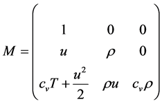
where

And 
One of the methods to solve a 1D nonlinear hyperbolic systems is the Godunov scheme
4.1. Godunov Scheme
Suppose we have subdivided our domain  in to N subintervals with
  and
and , so that
 .
.
Let us define . Assume
  at time
  is known and that
  is piecewise constant on
 . Then we solve exactly the local Riemann problem for
  on
on  with initial condition

Let us denote the solution by . Then the solution
  of the local Riemann problems are used to define the global solution v as

Then the solution  is defined by

Conservation form:
Since v is an exact solution on , we have


where  is constant for

With the numerical flux

This scheme is called Godunov scheme.
Solving a Riemann problem exactly is not always an easy task. Then we may need to consider an approximate solution of the Riemann problem.
4.2. Riemann Problem for a Linear System
Suppose we have a linear system  with initial condition
Let  are the eigenvalues and
  are the corresponding eigenvectors. Define
  such that

Then the solution of the Riemann problem is given by

where

A variety of approximate Riemann solvers have been proposed that can be applied more easily than the exact Riemann solver. One of the most popular Riemann solvers currently in use is due to Roe.
Godunov scheme with Roe approximation.
The idea is to replace the non-linear Riemann problem solved at each interface by an approximate one.

where  and
and  are the left and right values and
  satisfies

 is diagonalizable with real eigenvectors.
 as
as 
Conservation form of the Roe scheme.
The Roe scheme can be written in conservation form as

where

where  and
and  are the eigenvalues and eigenvectors of
  and
and .
.
The main task in the Roe scheme is the determination of the matrix of linearization A.
Now let us consider our equation (28) together with an equation of state of the form .
.
Then we approximate this non-linear system with an approximate linear system as follows:
Define  where
where

And


 is the specific enthalpy. These averages are called the Roe mean values.
  satisfies the
Roe conditions.
To solve our problem with the Roe scheme, we need to calculate the eigenvalues and their eigenvectors of the Jacobian matrix  which are needed to compute the Roe flux. But for complex EOS the determination of these eigenvectors may not be simple. One way of determining the eigenvectors of this Jacobian is by expressing the Euler equation in terms of primitive variables
 . We choose the temperature T as one of primitive variables than the pressure p, because in most equation of state p is expressed in terms of T.
Let  be the Euler equation in terms of the primitive variables V and
  be in conservative variables. The approximate linear system is


where 

Þ the matrices B and  have identical eigenvectors.
Further more, if  then
then . Then
  is the right eigenvectors of
4.3. Solving Euler Equation Using the Ideal Gas Law
In this section we solve one dimensional Euler equation with Ideal gas EOS. Consider the Euler equation (28) with the ideal gas law .
.
Using (21), the change of internal energy is given by  which implies
 , and the total energy
 is given by:
 .
.
Now let us express (28) in terms of the primitive variables , so that we can apply the Roe scheme easily.
Continuity equation:


Momentum equation:


Now using ,
,  , and
, and , the momentum equation in terms of the primitive variables is

Energy Equation:


 (29)
(29)
Now, using ,
,  , and
, and , the coefficient of
  in Equation (29) becomes
and the coefficient of  is 0.
is 0.
Then equation (29) reduces to
 (30)
(30)
Then the Euler equation in primitive variables is written as
 (31)
(31)
Or in vector form

Eigenvalues and eigenvectors of the coefficient matrix B of (31) are computed as follows.


where the local speed of sound c is given by

The matrix of the corresponding eigenvectors is:

To compute the eigenvectors of the Jacobian  we need to compute the matrix
  where
where  and
and 

Hence
The matrix R of eigenvectors of  is given by:

Since the total specific enthalpy h is given by  we can write the eigenvectors in terms of h as

4.4. Solving Euler Equation Using the Van der Waals (VDW) EOS
Here we solve one dimensional Euler equation with VDW EOS. Consider again the euler equation (28) with
VDW EOS  where
where  and
and , R is gas constant,
  critical pressure,
  critical temperature, and
  is the reduced temperature.
Again using (21), the change of internal energy is given by:

Here,  ,
,  , and
, and .
.
Integrating the above differential equation gives the internal energy .
.
The total energy  is given by:

Now let us express (28) in terms of the primitive variables 
Continuity equation:


Momentum equation:


Here,  ,
,  , and
, and .
.
Hence the momentum equation is reduced to

Energy Equation:


 (32)
(32)
Using ,
,  , and
, and .
.
The coefficient of  in (32) becomes

and the coefficient of  is 0.
is 0.
Then (32) reduces to
 (33)
(33)
The Euler equation is written as
 (34)
(34)
where ,
,  , and
, and .
.
Eigenvalues and eigenvectors of the coefficient matrix B of (34) are computed as follows.


where the local speed of sound c is defined as

The matrix of the corresponding eigenvectors is:

To compute the eigenvectors of the Jacobian  we need to compute the matrix
  where
where  and
and 

Hence

The matrix R of eigenvectors of  is given by:

where  and
and 
Since the total specific enthalpy h is given by  we can write the eigenvectors in terms of h as

where .
.
4.5. Solving Euler Equation Using the Soave-Redlich-Kwong (SRK) EOS
Let us consider (28) with SRK EOS

where ,
,  ,
,  ,
,  , w
, w
is the accentric factor R is gas constant,  critical pressure,
  critical temperature, and
  is the reduced temperature.
The internal energy is given by:


where .
.
After integrating the differential equation of the internal energy, we get

The total energy  is given by:

Continuity equation:


Momentum equation:


using ,
,  , and
, and  the
the
momentum equation is written as

Energy Equation:


 (35)
(35)


The coefficient of  in Equation (35) becomes

And the coefficient of  is 0.
is 0.
Notations: Let  denote the coefficient of
  and
and  denote the coefficient of
  i.e.
i.e.

Then Equation (35) reduces to
 (36)
(36)
The Euler equation is written as
 (37)
(37)
where,


Eigenvalues and eigenvectors of the coefficient matrix A of Equation (37) are given as follows.


where

The matrix of the corresponding eigenvectors is:

To compute the eigenvectors of the Jacobian  we need to compute the matrix
  where
where  and
and 

Hence

where 
And 
The matrix R of eigenvectors of  is given by:

Since the specific enthalpy h is given by  we can write the eigenvectors in terms of h as

where .
.
4.6. Solving Euler Equation Using the Peng-Robinson (PR) EOS
Let us consider (28) with PR EOS.

where ,
,  ,
,  ,
,
 , w is the accentric factor R is gas constant,
  critical pressure,
  critical temperature, and
 is reduced temperature.
The internal energy is given by:

Here,


where .
.
Integrating the above differential equation for internal energy we get

The total energy  is given by:

Continuity equation:


Momentum equation:

Using the continuity equation, it is reduced to

Here,  ,
,  , and
, and
 .
.
The momentum equation is written as

Energy Equation:


 (38)
(38)
Using


And

The coefficient of  in (38) becomes

And the coefficient of  is 0.
is 0.
Notations: Let  denote the coefficient of
  and
and  denote the coefficient of

Then (38) reduces to
 (39)
(39)
The Euler equation is written as
 (40)
(40)
where,


where

The matrix of the corresponding eigenvectors is:
To compute the eigenvectors of the Jacobian  we need to compute the matrix
  where
where  and
and 

Hence

where 
and .
.
The matrix R of eigenvectors of  is given by:

Since the specific enthalpy h is given by  we can write the eigenvectors in terms of h as

where .
.
4.7. Solving Euler Equation Using the Benedict-Webb-Rubin-Starling (BWRS) EOS
Let us consider (28) with BWRS EOS.

The internal energy is given by:


The total energy  is given by:

Continuity equation:


Momentum equation:


Let


The momentum equation is written as

Energy Equation:


 (41)
(41)


The coefficient of  in Equation (41) becomes

and the coefficient of  is 0.
is 0.
Notations: Let  denote the coefficient of
  and
and  denote the coefficient of
  i.e,
i.e, 
Then (41) reduces to
 (42)
(42)
The Euler equation is written as
 (43)
(43)
where,

Eigenvalues and eigenvectors of the coefficient matrix B of Equation (43) are computed as follows.


where

The matrix of the corresponding eigenvectors is:

To compute the eigenvectors of the Jacobian  we need to compute the matrix
  where
where  and
and 

Hence

where

and 
The matrix R of eigenvectors of  is given by:

Since the specific enthalpy h is given by  we can write the eigenvectors in terms of h as

where .
.
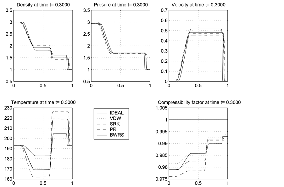
Figure 1. The results obtained by solving the homogeneous Euler equation by employing the ideal gas law and the other four equation of states.
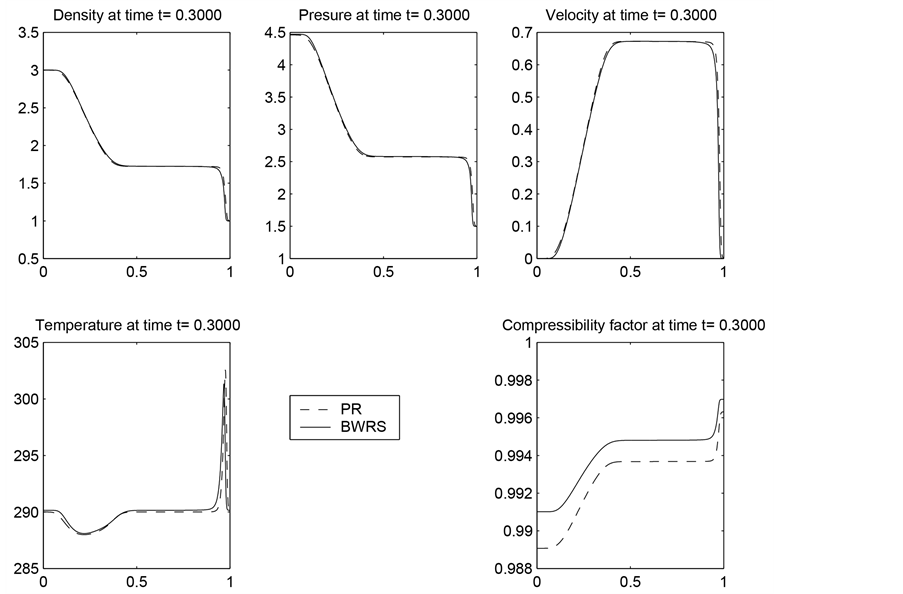
Figure 2. The results obtained by solving the Euler equation (including the source term) by employing the PR and BWRS EOS.
4.8. Application of the Roe solver
Now to apply the Roe scheme on (28), on each cell , we approximate the system by


where  and
and  is determined from the Roe averages. The solution is determined as:

where
where  and
and  are the eigenvalues and eigenvectors of
  and
and .
.
The last equation is a system of simultaneous algebraic equations for the variables .
.
The conservative variables  are determined by the scheme. The velocity is obtained from
  and
and . But to determine the value of the temperature T we use an iteration method (especially for the cases of complex EOS). Then the pressure P is computed from the EOS
4.9. Numerical Results
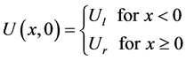
In this section we present some numerical results. We consider a tube of length 1, filled by Methane gas, the initial discontinuity is located at . In our simulation the following initial data is used.
 ,
,  ,
,  for
for 
 ,
,  ,
,  for
for .
.
In Figure 1, we have plotted the density, pressure, velocity, temperature, and the real gas compressibility factor computed by using each of EOS we discussed.
Figure 2 depicts results of (6), i.e, the Euler equation with the source term included, obtained by applying PR, and BWRS EOS.
5. Conclusion
The model that describes the flow of gas in a pipe is presented. Simplifications to the equations are made using appropriate assumptions. Several Equations of states that close the system of equations are examined and the results obtained for each equation of state are compared.
Cite this paper
Agegnehu Atena,Tilahun Muche, (2016) Modeling and Simulation of Real Gas Flow in a Pipeline. Journal of Applied Mathematics and Physics,04,1652-1681. doi: 10.4236/jamp.2016.48175
References
- 1. Feistauer, M. (1993) Mathematical Methods in Fluid Dynamics. Longman Scientific & Technical, New York.
- 2. Chorin, A.J. and Marsden, J. E. (1993) A Mathematical Introduction to Fluid Mechanics. Springer, New York.
http://dx.doi.org/10.1007/978-1-4612-0883-9 - 3. LeVeque, R.J. (1990) Numerical Methods for Conservation Laws, Lectures in Mathematics. ETH Zuerich, Birkhaeuser, Basel.
http://dx.doi.org/10.1007/978-3-0348-5116-9 - 4. Kroener, D. (1997) Numerical Schemes for Conservation Laws/John Wiley & Sons Ltd, England and B.G. Teubner, Germany.
- 5. Modisette, J.L. (2000) Equations of State Tutorial. 32nd Annual Meeting PSIG (Pipeline simulation Interest Group), Savanah, Georgia.
- 6. Starling, K.E. (1973) Fluid Thermodynamic Properties for Light Petroleum Systems. Gulf Publ., Houston.