Theoretical Economics Letters
Vol.2 No.5(2012), Article ID:25808,8 pages DOI:10.4236/tel.2012.25089
On the Identification of Technology Shocks: An Alternative to the Standard Long-Run Method
Department of Economics, University of Colorado, Boulder, USA
Email: demirel@colorado.edu
Received September 11, 2012; revised October 13, 2012; accepted November 15, 2012
Keywords: Technology Shocks; Long-Run Restrictions; Relative Identification
ABSTRACT
This study proposes an alternative procedure to identify technology shocks using vector autoregressions (VARs). The proposed procedure delivers improved small-sample properties relative to the standard long-run identification method provided that the dynamics of the observed variables can only be captured precisely by an infinite-order VAR. Monte Carlo experiments on artificial data produced by a standard version of the real business cycle model demonstrate that the proposed procedure is associated with smaller average bias and mean square error. These results obtain under a range of specifications regarding the share of technology shocks in overall output variability.
1. Introduction
In the real business cycle (RBC) literature, technology shocks are frequently identified by implementing long-run restrictions in structural vector-autoregressions (VARs) (see, e.g. [1-3]). A number of recent studies have called into question the plausibility of identifying technology shocks by imposing long-run restrictions on VARs. Demirel [4], Mertens [5], and Chari et al. [6] find that the standard long-run identification approach can be highly inaccurate if the number of lags included into the estimated VAR is smaller than the number of lags involved with the actual data-generating process. Since in many RBC models the reduced-form dynamics of the observed variables can only be captured by an infinite-order VAR, this type of mismatch between the estimated and actual lag structures is often relevant (see [6-9]). In this paper, I propose an alternative identification procedure that is designed to reduce the lag-truncation bias that emerges in the presence of this mismatch. I show that, in the estimation of the impact response of labor to a technology shock, the proposed procedure is associated with smaller average bias and mean square error relative to the standard long-run identification method.
To implement long-run restrictions in structural VARs, one needs an estimate for the zero-frequency spectral density of the data. Christiano et al. [10,11] show that the standard long-run method uses a particular estimate of the zero-frequency density that is based on the OLS estimate of the sum of VAR coefficients. In the presence of a lag-truncation-type mismatch between the estimated and actual VARs, the OLS-based estimate of the sum of VAR coefficients can be highly biased. Christiano et al. [10] argue that the poor performance of the standard long-run identification procedure is primarily due to this bias involved with the OLS estimate of the sum of VAR coefficients and suggest considering non-parametric methods to estimate the zero-frequency spectral density of the data. Using Monte Carlo simulations, they find that their non-parametric procedure (henceforth, the CEV method) outperforms the standard OLS-based long-run identification scheme under some reasonable parameterizations of the RBC model.
The motivation for the proposed procedure emerges upon an assessment of the consequences of adopting a misspecified VAR to identify technology shocks. Experiments on artificial data produced by estimated versions of the RBC model show that, in the presence of lag-truncation bias, the standard estimation procedure with long-run restrictions delivers a shock that explains too much of the short-run variance of labor productivity and aggregate employment relative to the true technology shock of the RBC model. The discrepancy worsens as the share of non-technology shocks in overall output variability increases. Motivated by this observation, I suggest identifying technology shocks on the basis of the difference between the long-run and short-run forecast revision variances they generate. More specifically, I propose focusing on the disturbance for which the explained fraction of labor productivity's long-run variance is as great as possible relative to the explained fraction of the shortrun variances of labor productivity and aggregate employment. The proposed procedure selects the shock that drives as much as possible of the long-run variation of labor productivity while explaining as least as possible of the short-run variation. In this sense, it is expected to counteract the tendency of the standard method to deliver a shock that overshoots the short-run variability of the VAR variables. Following Uhlig [12], I use principal components analysis to determine the shock that satisfies this property.
Using Monte Carlo simulations, I evaluate the performance of the proposed method relative to the standard long-run and the CEV procedures. In a series of simulation experiments, I produce artificial data sequences using the most commonly adopted parameterizations of the RBC model. Then, I apply the proposed procedure as well as the standard long-run and the CEV methods to each simulated data sequence to recover technology shocks. I consider two different VAR specifications in which hours worked is entered into the VAR in first differences and in levels. I find that, in the estimation of the contemporaneous response of labor to a technology shock, the proposed method outperforms the standard long-run and the CEV methods in terms of average bias and mean square error.
The remainder of the paper is organized as follows: Section 2 discusses the identification procedures based on long-run restrictions. Section 3 outlines the proposed method and describes its implementation. Section 4 evaluates the performance of the proposed approach relative to the standard long-run and the CEV method using Monte Carlo simulations. Section 5 summarizes the main results and concludes.
2. Identifying Technology Shocks with Long-Run Restrictions
2.1. The Standard Long-Run Method
As discussed in Gali [13], in a large class of real business cycle (RBC) models, long-run variability of labor productivity is exclusively driven by technology shocks. This distinguishing property is referred to as the exclusion restriction. Furthermore, in the standard RBC framework, the impact of a positive technology shock on labor productivity is positive in the long-run. This property, in turn, implies a sign restriction. Exclusion and sign restrictions can be exploited to identify technology shocks using a VAR(m) specification of the form
 (1)
(1)
where
 (2)
(2)
and .
.
The vector Yt is often specified as

where  and
and  respectively denote average labor productivity and quasi-differenced percapita hours. Note that, in the case
 , aggregate employment enters
  in levels. This is the specification adopted by many studies including Christiano et al. [10,11], and will be among the cases I consider in the following analysis. Another common practice is to include the first-difference of aggregate employment into the VAR specification (by setting
 ). As shown by Chari et al. [6], in the case
 , a reduced-form VAR representation for
  ceases to exist in the RBC model. To circumvent this problem, they set the quasi differencing parameter to 0.99. In this case,
  admits an infinite-order VAR representation and the impulse response of labor productivity to a technology shock is indistinguishable from the case
 . I will also consider the case
  in the following analysis.
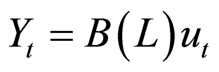
Given (1),  can be expressed in moving average form as follows:
 (3)
(3)
where 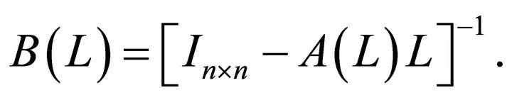 The mapping from the vector of structural disturbances,
  , to the vector of VAR innovations,
  , is conjectured to be of the form
 (4)
(4)
where . Without loss of generality, the technology shock can be assumed to rank first in
 . To evaluate the effects of a technology shock on
 , one needs to know
  as well as the first column of the matrix R, which will be denoted
 . The vector
  describes the contemporaneous effects of a technology shock on
  and is often referred to as the impact vector. The objects
  and Ω are typically estimated using OLS. To estimate
 , however, one needs to impose exclusion and sign restrictions.
Define . Given that the first element of
  is the technology shock, exclusion and sign restricttions imply that
  is of the form
 (5)
(5)
where  and the upper-right expression is a
  dimensional row vector of zeros. The form described by (5) implies that only technology shocks can influence labor productivity (the first element in
 ) in the long-run. The object
  can be identified using the zero-frequency spectral density matrix of
 . The standard long-run procedure uses the OLS estimates for
  and Ω to recover the zero-frequency density of
  as
as
 (6)
(6)
Once  is estimated using (6),
  can be identified as the matrix that factors
  as
as
Note that there are many ways in which the matrix  can be decomposed in the form
  . Yet, Christiano et al. [11] show that the decompositions of this form that are also consistent with the structure described by (5) all have the same first column. Therefore, a lower-triangular Cholesky decomposition can be applied to
  to obtain the estimate
 .
.
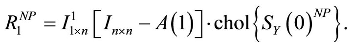
Then, using the estimate for  and the relationship
 , the impact vector of the technology shock can be recovered as
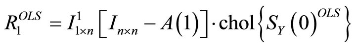 (7)
(7)
where  is a
is a  vector of all zeros but the 1st element is replaced with unity.
2.2. A Non-Parametric Alternative to the Standard Method
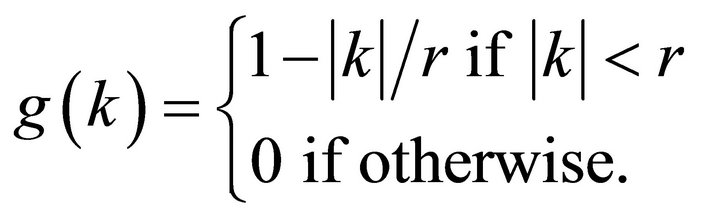
The standard long-run method is known to deliver imprecise estimates in the presence of VAR misspecification. Christiano et al. [10] argue that this is because the OLS-based estimate of the zero-frequency spectral density of  (given by 6) becomes highly inaccurate if the data-generating process is an infinite-order VAR. To remedy this problem, they suggest adopting a nonparametric approach to estimate the zero-frequency spectral density. In particular, they consider a Bartlett estimate of the form
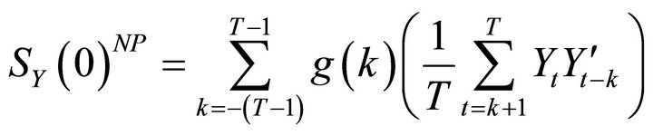 (8)
(8)
where
The procedure of Christiano et al. [10] involves replacing  with
with  and identifying the impact vector of the technology shock as
 (9)
(9)
Christiano et al. [10] show that, under certain relevant parameterizations of the RBC model, the non-parametric method (henceforth, CEV procedure) proves more successful relative to the standard method1. This is because,  accounts for some of the information
  is unable to capture due to lag-truncation and provides a more accurate estimate of the zero-frequency spectral density. However, Mertens [5] shows that the CEV procedure (fully described by 9) fails to properly utilize this additional information in the estimation of the impact vector. Consequently, the improved small-sample results of the CEV method do not extend to a wider range of parameterizations of the RBC model.
3. Relative Identification
3.1. Motivation
To motive the proposed identification approach, I next discuss the consequences of implementing the standard long-run identification procedure in the presence of VAR misspecification. Suppose that the true data-generating process is an infinite-order VAR of the form
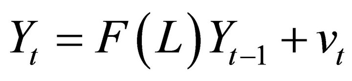 (10)
(10)
where
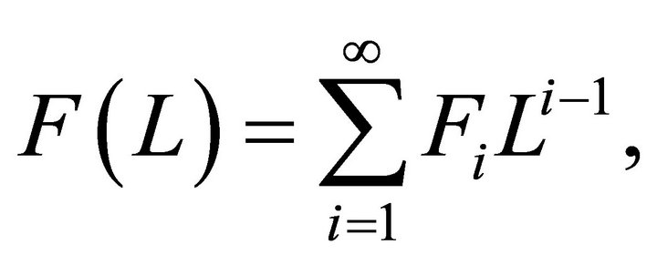
and . Note that any attempt to estimate (10) with a finite-order VAR of the form (1) will always result in a lag-truncation bias. Christiano et al. [10] show that the residual covariance matrix of the misspecified
  is related to the true residual covariance matrix
  through the following relationship:
 (11)
(11)
where
and ,
,  denote the lag polynomials
 ,
,  evaluated at
 . This equality follows immediately from the spectral domain representations of (1) and (10). According to (11), the OLS procedure selects the autoregressive matrices
  to minimize a quadratic form that measures the distance between the actual and fitted lag polynomials averaged across all frequencies weighted by the spectral density of
  at each frequency.
Equation (11) highlights two major consequences of adopting a misspecified VAR: 1—In the presence of a lag-truncation problem, the OLS procedure cannot be expected to deliver an accurate estimate for the sum of VAR coefficients unless the spectral density of  at zero frequency is large relative to non-zero frequencies. Thus, in general, we have
 . 2—Equation (11) also implies that
 , i.e.,
  is a positive semi-definite matrix. Thus, the estimates
  and Ω are both biased under VAR misspecification.
The main motivation for relative identification emerges upon an investigation of the implications of these biases on the short-run variances of labor productivity and aggregate employment the technology shock is found to drive using the standard long-run identification method. Figure 1 displays the percentage difference between the current-period forecast error variances the technology shock is estimated to explain in the artificial data (averaged across 1000 trials) and the true fraction the technology shock explains in the RBC model. It is observed that the shock identified using the standard long-run method overestimates the true values. This finding obtains under alternative scenarios regarding the share of technology shocks in overall output variability2. In all considered cases, the shock the standard long-run method yields overshoots the true fraction of short-run variances the technology shock explains in the RBC model. As Figure 2 attests, similar patterns obtain under the parameterization of the RBC model adopted by Chari et al. [6].
As discussed in the previous section, the standard long-run approach determines the disturbance that singlehandedly explains all of the infinite-period-ahead forecast revision variance of labor productivity. Demirel [4] shows that this is equivalent to determining the shock that explains on its own as much as possible of the long-run variance of labor productivity. Thus, the standard long-run identification procedure can be viewed as a version of the maximum share approach suggested by Francis et al. [15] and implemented in the frequency domain by DiCecio and Owyang [16].
Monte Carlo experiments reveal that, in the presence of lag-truncation bias, imposing this identifying restriction on the misspecified VAR yields a shock that tends to explain too much of the current-period forecast error variance of labor productivity and employment relative to the true technology shock.
To counter this tendency, I propose considering the disturbance for which the explained fraction of the infinite-period-ahead forecast variance of labor productivity is as great as possible relative to the explained fractions of the current-period forecast variances of labor productivity and employment. This procedure involves determining the disturbance for which the difference between the explained fractions of long-run and shortrun variances reaches a maximum. Thus, the procedure places a certain amount of weight on minimizing the currentperiod forecast revision variance the identified shock explains. Although this property does not perfectly overlap with the notion of a technology shock, in the presence of lag-truncation bias, the proposed adjustment to the long-run identifying assumption works against the tendency of the standard approach to overshoot the true short-run variances. This, in turn, results in a more accurate estimate for technology shocks.
3.2. Implementation
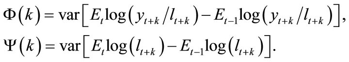
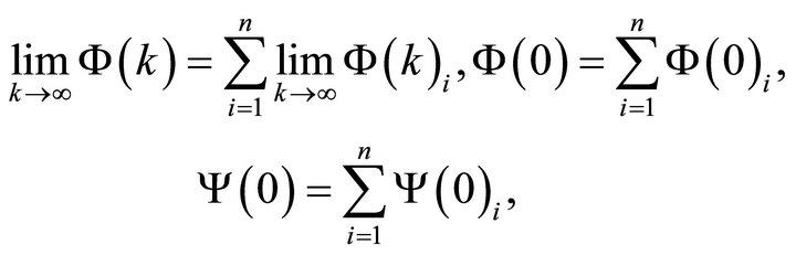
Define k-period-ahead forecast revision variances of labor productivity and employment as
Using (1) and (4), infinite-period-ahead forecast revision variance of labor productivity can be found as
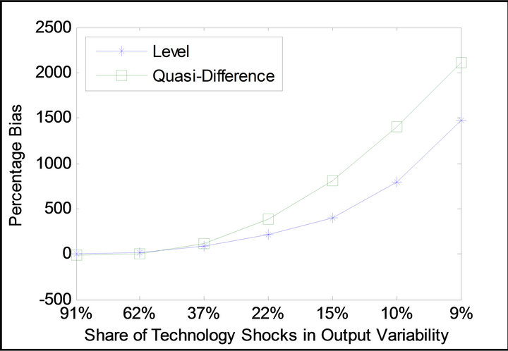
Figure 1. Standard long-run method’s bias profile in the estimation of short-run variances under the parameterization of Christiano et al. [11].
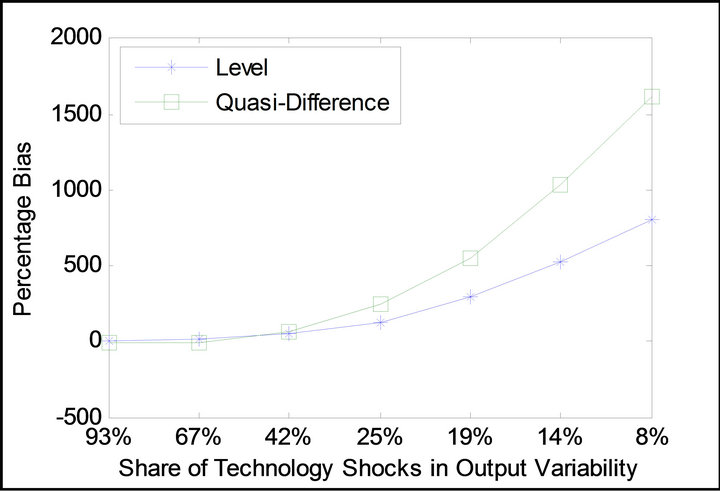
Figure 2. Standard long-run method’s bias profile in the estimation of short-run variances under the parameterization of Chari et al. [6].
 (12)
(12)
where  and
and is a
is a  vector of all zeros but the
  element is replaced with unity. Similarly, current-period forecast revision variances of labor productivity and aggregate employment can be respectively expressed as
 (13)
(13)
Using
expressions (12) and (13) and can be rewritten as
 (14)
(14)
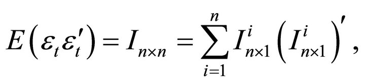
where
and . Expression (14) shows how infinite-period forecast revision variance of labor productivity and current-period forecast revision variances of labor productivity and employment can be decomposed into n elements each exclusively attributable to a particular structural disturbance in εt. Since the first element in εt corresponds to the technology shock, its contribution to the infinite-period forecast variance of
  is given by
 . Similarly, the contribution of the technology shock to the current-period forecast revision variances of
  and
and  are, respectively,
  and
and . Now, let’s define
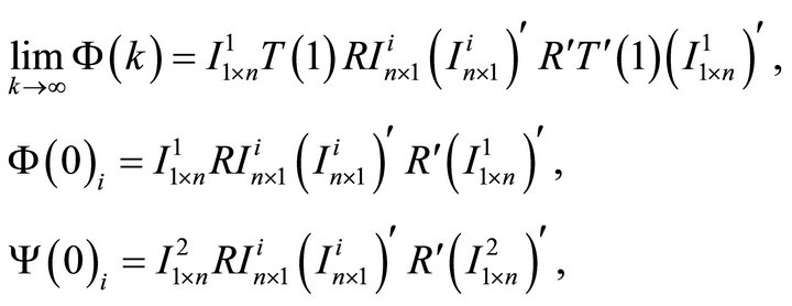
After obtaining estimates for the objects  and
and , relative identification procedure can be implemented as follows: Let P correspond to a lower-triangular Cholesky decomposition of Ω (i.e.,
 ). Given an orthonormal matrix Q (i.e.,
 ), a particular decomposition of the covariance matrix Ω can be obtained via the relationship
  where
where . Also note that one can write
  where
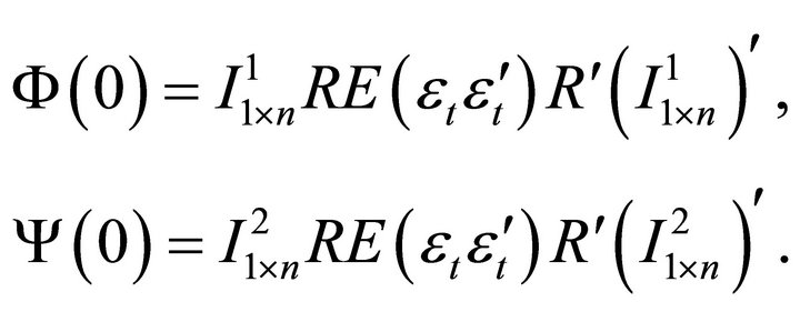
where  denotes the ith column vector of Q. It is shown in the appendix that the statistic
  can be expressed as
 (15)
(15)
where  is a
is a  matrix of all zeros but the ith-column jth-row element is replaced with unity. Relative identification involves determining the decomposition of the covariance matrix
  indexed by the Q for which the first column
  results in the maximum value (15) can achieve. Thus, the associated identification problem can be expressed as
 (16)
(16)
subject to
where, as suggested by (15),
The first constraint  ensures that
  belongs to an orthonormal matrix and the second constraint guarantees that the long-run effect of the identified shock on labor productivity is positive. As shown in Uhlig [12], the optimal value of
  (denoted
 ) that solves (16) is given by the eigenvector of Λ that corresponds to its greatest eigenvalue, i.e., the first principal component of Λ. Once
  is recovered by solving for the first princepal component of Λ, the impact vector of the technology shock can be estimated as
 (17)
(17)
Throughout the rest of the analysis, we shall compare the small-sample properties of the relative method described by (17) with those of the standard long-run and the CEV methods respectively described by (7) and (9).
4. Monte Carlo Experiments
To evaluate the performance of the proposed method, I next conduct a series of simulation exercises. In these experiments, I produce artificial data using the baseline RBC model adopted by Chari et al. [6] and Christiano et al. [11]. Since the model is standard, I shall skip the explanation of the full theoretical structure. It should however be noted that, in the standard RBC model, the equilibrium dynamics of the vector
can only be described accurately by an infinite-order VAR. Thus, using a finite-order VAR to identify technology shocks will always result in a lag-truncation bias, which will play a central role in the following experiments.
I consider two alternative parameterizations of the RBC model adopted by [6] and [11]3. These parameter choices render the results of the analysis immediately comparable with the results of the previous studies. In addition, I consider a range of scenarios regarding the share of technology shocks in overall output variability. Following the rest of the literature, for each alternative specification, I simulate 1000 data sequences each of length T = 240 quarters. Then, I run a VAR with 4 lags on each of these 1000 data series and identify technology shocks using the proposed method as well as the standard long-run and the CEV methods. In all exercises, I estimate a bivariate VAR of the form
 .
.
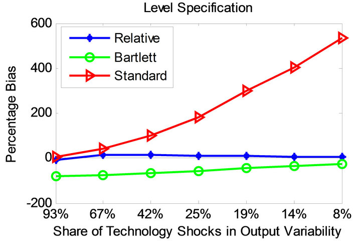
First, I focus on the average bias associated with each method in the estimation of the impact coefficient of labor. The impact coefficient of labor corresponds to the contemporaneous percentage response of employment to a one-standard-deviation technology shock. Average bias is defined as the percentage difference between the true impact coefficient in the RBC model and the average of all estimated impact coefficients across simulations.
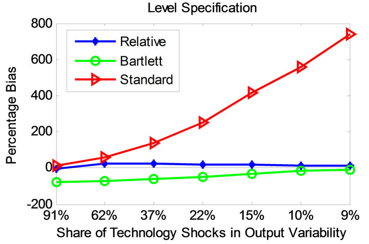
Figures 3 and 4 display the bias profile of each identification method under the parameterizations of Christiano et al. [11] and Chari et al. [6] for level and quasidifference specifications. Observe that the average bias associated with the relative identification method is much smaller compared to the other methods in all considered cases.
The standard long-run method becomes more accurate as the share of technology shocks in overall output variability increases. As the share of technology shocks becomes smaller, the standard method turns less accurate. This does not appear to be the case for the CEV method. Compared to the relative method, however, the CEV method proves less successful.
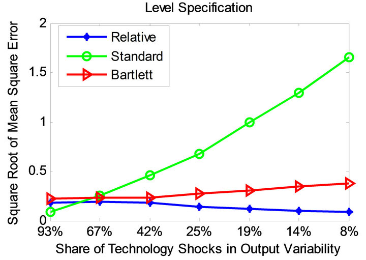
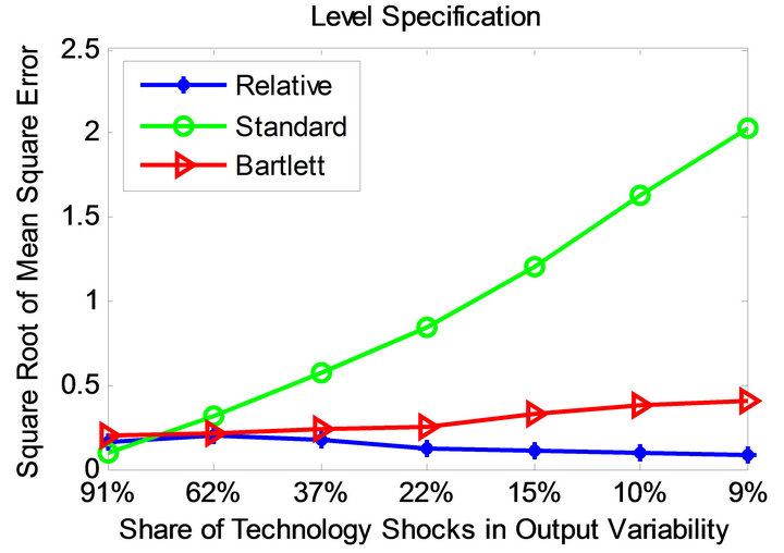
Figures 5 and 6 demonstrate the root mean square error profiles under the parameterizations adopted by Christiano et al. [11] and Chari et al. [6] for level and quasidifference specifications. Root mean square error statistic measures average bias and sampling uncertainty simultaneously. It is defined as
where xi denotes the impact coefficient estimate obtained from the ith experiment and x is the true value of the impact coefficient.
Observe that the relative method is also associated with significantly smaller mean square error compared to the standard long-run and CEV procedures. This appears to be the case for all considered parameterizations and volatility specifications.
 (a)
(a)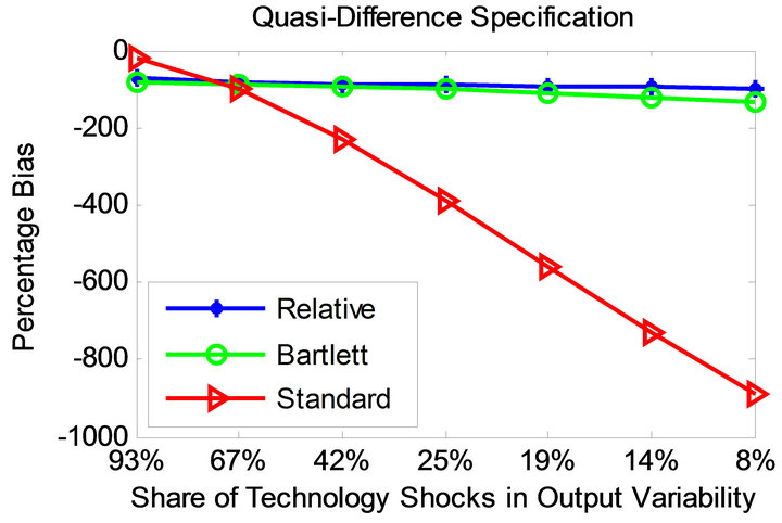 (b)
(b)
Figure 3. Bias profiles under the parameterization of [11].
 (a)
(a)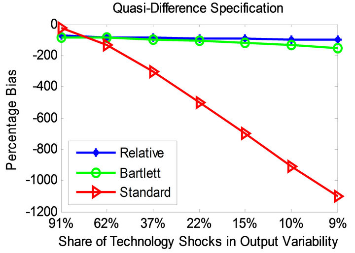 (b)
(b)
Figure 4. Bias profiles under the parameterization of [6].
 (a)
(a)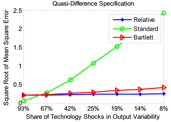 (b)
(b)
Figure 5. Mean square error profiles under level and quasidifference specifications (parameterization of [11]).
 (a)
(a)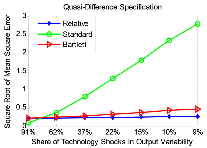 (b)
(b)
Figure 6. Mean square error profiles under level and quasidifference specifications (parameterization of [6]).
5. Concluding Remarks
This study suggests an alternative approach to identify technology shocks using VARs. I test the performance of the proposed method by applying it to artificial data generated by the standard RBC model. I evaluate the smallsample performance of the proposed procedure by recovering technology shocks from simulated time-series data that are produced by a standard version of the RBC model. I consider alternative parameterizations of the RBC model as well as a range of specifications regarding the share of technology shocks in overall output variability. Monte Carlo experiments on simulated data reveal that the proposed method delivers considerably improved small-sample properties than the standard long-run identification method widely adopted in the literature and its non-parametric version proposed by [11]. In particular, it significantly reduces the average bias and mean square error in the estimation of the impact coefficient of labor.
It is important to note that this study assesses the small-sample properties of the proposed relative identification approach for a specific range of data-generating processes. Since the small-sample performance of an estimation procedure depends on the properties of the underlying data-generating process, one should be cautious generalizing the results. At the very least, the findings suggest that the relative approach can identify technology shocks far more accurately provided that the data-generating process is the standard RBC model.
REFERENCES
- N. Francis and V. A. Ramey, “Is the Technology-Driven Real Business Cycle Hypothesis Dead? Shocks and Aggregate Fluctuations Revisited,” Journal of Monetary Economics, Vol. 52, No. 8, 2005, pp. 1379-1399. doi:10.1016/j.jmoneco.2004.08.009
- N. Francis and V. A. Ramey, “Measures of Per Capita Hours and Their Implications for the Technology-Hours Debate,” Journal of Money, Credit and Banking, Vol. 41, No. 6, 2009, pp. 1071-1097. doi:10.1111/j.1538-4616.2009.00247.x
- J. Gali and P. Rabanal, “Technology Shocks and Aggregate Fluctuations: How Well Does the RBC Model Fit Postwar US Data?” NBER Macroeconomics Annual, Vol. 19, 2004, pp. 225-288.
- U. D. Demirel, “Identification of Technology Shocks Using Misspecified VARs,” University of Colorado, Boulder, 2012.
- E. Mertens, “Are Spectral Estimators Useful for Implementing Long-Run Restrictions in SVARs?” Journal of Economic Dynamics and Control, Vol. 36, No. 12, 2012, pp. 1831-1842. doi:10.1016/j.jedc.2012.06.007
- V. V. Chari, P. J. Kehoe and E. L. McGrattan, “Are Structural VARs with Long-Run Restrictions Useful in Developing Business Cycle Theory?” Journal of Monetary Economics, Vol. 55, No. 8, 2008, pp. 1337-1352. doi:10.1016/j.jmoneco.2008.09.010
- C. J. Erceg, L. Guerrieri and C. Gust, “Can Long-Run Restrictions Identify Technology Shocks?” Journal of the European Economic Association, Vol. 3, No. 6, 2005, pp. 1237-1278. doi:10.1162/154247605775012860
- F. Ravenna, “Vector Autoregressions and Reduced Form Representations of DSGE Models,” Journal of Monetary Economics, Vol. 54, No. 7, 2007, pp. 2048-2064. doi:10.1016/j.jmoneco.2006.09.002
- T. F. Cooley and M. Dywer, “Business Cycle Analysis without Much Theory: A Look at Structural VARs,” Journal of Econometrics, Vol. 83, No. 1-2, 1998, pp. 57- 88. doi:10.1016/S0304-4076(97)00065-1
- L. Christiano, M. Eichenbaum and R. Vigfusson, “Alternative Procedures for Estimating Vector Autoregressions Identified with Long-Run Restrictions,” Journal of the European Economic Association, Vol. 4, No. 2-3, 2005, pp. 475-483. doi:10.1162/jeea.2006.4.2-3.475
- L. Christiano, M. Eichenbaum and R. Vigfusson, “Assessing Structural VARs,” NBER Macroeconomics Annual, Vol. 21, 2006, pp. 1-72.
- H. Uhlig, “What Moves Real GNP?” Humboldt University, Berlin, 2003.
- J. Gali, “Technology, Employment, and the Business Cycle: Do Technology Shocks Explain Aggregate Fluctuations?” American Economic Review, Vol. 89, No. 1, 1999, pp. 249-271. doi:10.1257/aer.89.1.249
- D. W. K. Andrews and J. C. Monahan, “An Improved Heteroskedasticity and Autocorrelation Consistent Covariance Matrix Estimator,” Econometrica, Vol. 60, No. 4, 1992, pp. 953-966. doi:10.2307/2951574
- N. Francis, M. T. Owyang, J. E. Roush and R. DiCecio, “A Flexible Finite-Horizon Alternative to Long-Run Restrictions with an Application to Technology Shocks,” Federal Reserve Bank of St. Louis Working Paper 2005- 024F, 2010.
- R. DiCecio and M. T. Owyang, “Identifying Technology Shocks in the Frequency Domain,” Federal Reserve Bank of St. Louis Working Paper 2010-025A, 2010.
Appendix
In the reduced-form VAR described by (1) we have . Thus, the infinite-period-ahead forecast revision variance of labor productivity described by (12) can be rewritten as
 (18)
(18)
where . Similarly, current-period forecast revision variances of labor productivity and aggregate employment can be respectively written as
 (19)
(19)
Now using (18) and (19), the statistic can be obtained as
 (20)
(20)
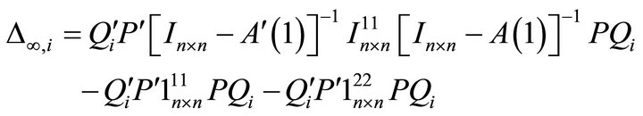
Let  denote a
  matrix of all zeros but the ith-column jth-row element is replaced with unity. Then, (20) can be reexpressed as

which brings us to (15) in the text.
NOTES
1Christiano et al. [10] also evaluate an alternative non-parametric estimator of the zero-frequency spectral density suggested by Andrews and Monahan [14]. They find that the small-sample performances of the Bartlett and Andrews-Monahan estimators are very close.
2Output variance in these experiments is computed using simulated band-pass filtered data sequences of length 50,000 quarters.
3See Chari et al. [6] and Christiano et al. [11] (or Demirel [4]) for a list of adopted parameter values.