Journal of Mathematical Finance
Vol.2 No.1(2012), Article ID:17606,16 pages DOI:10.4236/jmf.2012.21013
A Skewness-Adjusted Binomial Model for Pricing Futures Options—The Importance of the Mean and Carrying-Cost Parameters
1Department of Finance, Xavier University, Cincinnati, USA
2Department of Economics, Xavier University, Cincinnati, USA
Email: {johnsons, sen, balyeatb}@xavier.edu
Received October 16, 2011; revised December 2, 2011; accepted December 10, 2011
Keywords: Options Pricing; Black-Scholes; Skewness
ABSTRACT
In this paper, we extend the Johnson, Pawlukiwicz, and Mehta [1] skewness-adjusted binomial model to the pricing of futures options and examine in some detail the asymptotic properties of the skewness model as it applies to futures and spot options. The resulting skewness-adjusted futures options model shows that for a large number of subperiods, the price of futures options depends not only on the volatility and mean but also on the risk-free rate, asset-yield, and other carrying-cost parameters when skewness exists.
1. Introduction
One of the interesting, as well as subtle, features of the Black-Scholes (B-S) [2] model and the binomial option pricing model (BOPM) with a large number of subperiods (n) is that the models depend only on the variance. In these models, the mean is not important in determining the value of spot options and the mean and net carry cost are not important for futures options. These implications of the model, however, depend on the assumption that the logarithmic return of the underlying security is normally distributed. Studies by Johnson, Zuber, and Gandar [3] and [4] have shown that in periods of increasing stock prices or rates, the logarithmic return of stock indexes and interest rates are often characterized by a positive mean and significant negative skewness, and in periods of decreasing prices or rates, the logarithmic returns are often characterized by a negative mean and significant positive skewness. Moreover, several earlier empirical studies have reported that the B-S model consistently underprices options in the presence of skewness; see for instance, Stein and Stein [5], Wiggins [6], and Heston [7].
Jarrow and Rudd [8] and Corrado and Tie Su [9] have extended the B-S model to account for cases in which there is skewness in the underlying security’s return distribution. Similarly, Câmara and Chung [10] and Johnson, Pawlukiewicz, and Mehta (JPM) [1] have extended the Cox, Ross, and Rubinstein (CRR) [11] and Rendleman and Bartter (RB) [12] binomial option pricing model to include skewness. In their paper, JPM also show that skewness changes the asymptotic properties of the up (u) and down (d) parameters, elevating the relative importance of the mean in valuing options. This property of their skewness model suggests that when distributions of logarithmic returns are characterized by skewness, the observed pricing biases associated with the B-S model may be due to not only the omission of skewness, but also the mean.
Today, the derivative market for non-stock options (indices, currencies, debt securities, and commodities) is dominated more by options on futures contracts than options on spot securities. The purpose of this paper is to extend the JPM skewness-adjusted binomial model to the pricing of futures options. In addition, given that one of the features of the JPM skewness model for spot options is that skewness changes the asymptotic properties of the u and d parameters, this paper examines in some detail the asymptotic properties of the skewness-adjusted binomial model as it applies to both futures and spot options. Our results show that the skewness model for futures options has similar asymptotic properties as the model for spot options. However, in the case of futures options, the presence of skewness elevates the importance of the mean, as well as the risk-free rate, the asset yield, and other parameters that are defined by the carrying-cost model.
2. Binomial Futures Options Pricing Model
The standard binomial option model values futures options recursively by determining the futures option’s intrinsic values at expiration and then using the singleperiod binomial model at each node to price the futures option equal to the value of its replicating portfolio:
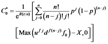 (1)
(1)
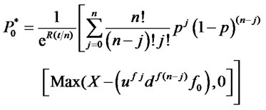 (2)
(2)
where:
C0 = call price P0 = put price R = annual risk-free rate t = time to expiration expressed as a proportion of a year X = exercise price f0 = current futures price uf = the futures up parameter df = the futures down parameter n = number of periods to the option’s expiration t/n = length on the binomial period = time to expiration as a proportion of a year (t) divided by number of periods to the option’s expiration p = risk-neutral probability For the case of an option on a financial futures contract (e.g., index, currency, or debt security) in which the underlying security is adjusted to reflect a continuous asset yield (e.g., dividend yield, foreign risk-free rate, or coupon rate), the equilibrium futures price as determined by the carrying-cost model is:
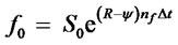 (3)
(3)
where:
S0 = current spot price
ψ = annual asset yield
∆t = t/n = length of binomial steps as a proportion of a year nf = number of discrete binomial periods of length ∆t to the futures’ expiration The risk-neutral probability, p, for options on financial futures defined in terms of the up and down parameters for the underlying spot (u = Su/S0 and d = Sd/S0, where Su = uS0 and Sd = dS0) is:
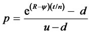 (4)
(4)
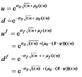
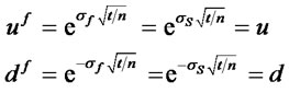
If the carrying-cost model holds, then the up and down parameters for the futures price (uf = fu/f0 and df = fd/f0, where fu = uf and fd = df0) are given as:
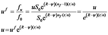 (5)
(5)
 (6)
(6)
Substituting Equations (5) and (6) into Equation (4), the risk-neutral probability for futures call and put option prices can be alternatively defined in terms of the futures up and down parameters (uf and df) :
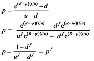 (7)
(7)
2.1. Skewness-Adjusted Formulas for uf and df
In their seminal 1979 paper, Cox, Ross, and Rubinstein [11] derive the formulas for estimating the u and d parameters of the BOPM for a spot option. They do this by setting the equations for the expected value and variance of the logarithmic return of the underlying security equal to their empirical values. The resulting equations are then solved simultaneously for u and d under the assumption that the probability of the underlying security increasing in one period (q) is 0.5. By treating q as an unknown, JPM extend the CRR binomial model to include skewness. Specifically, in the JPM skewness-adjusted model, the u, d, and q values that define a binomial process for a spot security are found by setting the equations for the expected value, variance, and skewness equal to their respective empirical values and then solving the resulting equation system simultaneously for u, d, and q. That is:
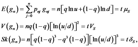 (8)
(8)
where:
g = logarithmic return of the underlying spot price = ln(S1/S0)
j = number of increases in n periods pnj = probability of j increases in n periods, where:
mS, VS, σS, dS = the annualized empirical values of the mean, variance, standard deviation, and skewness of the spot price’s logarithmic return t = time to expiration as a proportion of a year n = number of periods The values of u, d, and q that satisfy this system of equations are:
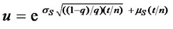 (9)
(9)
 (10)
(10)
 (11)
(11)
For futures options, the formulas for estimating uf, df, and q are found by setting the equations for the population moments for the futures price’s logarithmic return equal to their respective empirical values, and then solving the resulting equation system simultaneously for uf, df, and q:
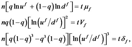 (12)
(12)
where mf, Vf, σf, and df are respectively the annualized empirical values of the mean, the variance, the standard deviation, and skewness of the futures price’s logarithmic return, ln(f1/f0), and t is the time to expiration as a proportion of a year.
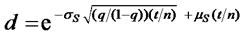
The values of uf, df, and q that satisfy this system of equations are:
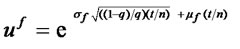 (13)
(13)
 (14)
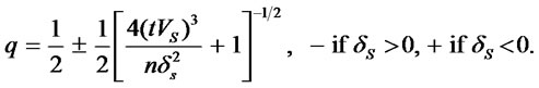
(14)
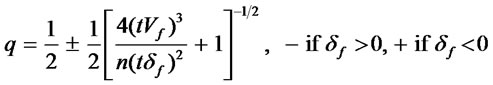 (15)
(15)
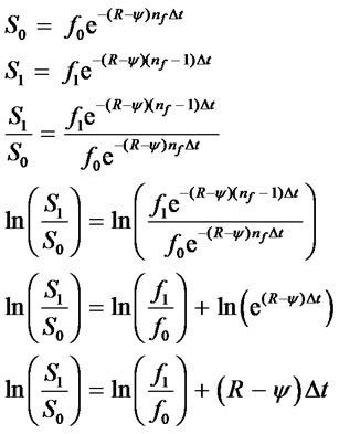
2.2. Relations between Futures and Spot Mean and Volatility
The relationships between the spot and futures parameters follow directly from the futures and spot relation defined by the carrying-cost model given in equation (3). Specifically, from equation (3), one can solve the relationship between the spot and futures moments as follows:
 (16)
(16)
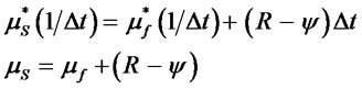
Taking the expected value of both sides of Equation (16) results in the mean over a period of time ∆t:
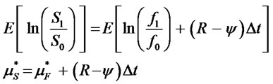
where  and
and  are respectively the periodic means of a spot option and a futures option for a period of length ∆t( = t/n). Multiplying both sides by 1/∆t results in the annualized means (µS and µF):
Taking the variance of both sides of (16) and annualizing we obtain:
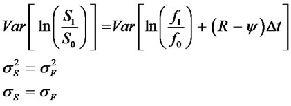
A similar proof shows that δS = δF.
Thus, the relationships between the mean, standard deviation, and skewness on the futures and spot logarithmic returns are:
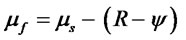 (17)
(17)
 (18)
(18)
 (19)
(19)
Substituting (17) and (18) into equations (13) and (14), uf and df can be expressed in terms of the spot mean and variability, the risk-free rate, and the asset yield:
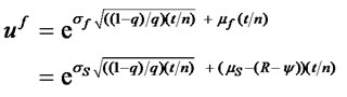 (20)
(20)
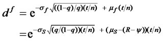 (21)
(21)
The difference between the futures up and down parameters (uf and df respectively), and the spot up and down parameter (u and d respectively (see Equations (9) and 10)) is the net cost of carry term (R – ψ). If R > ψ, then the futures market is normal with the futures price (equation (3)) exceeding the spot.
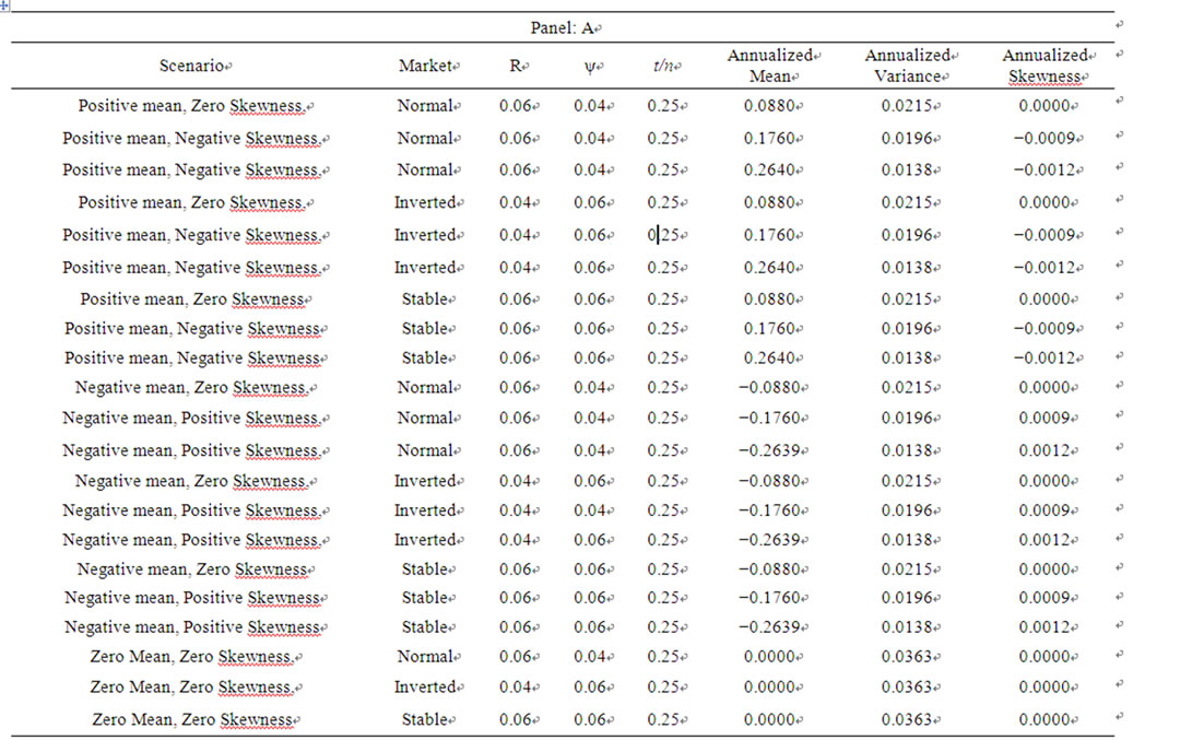
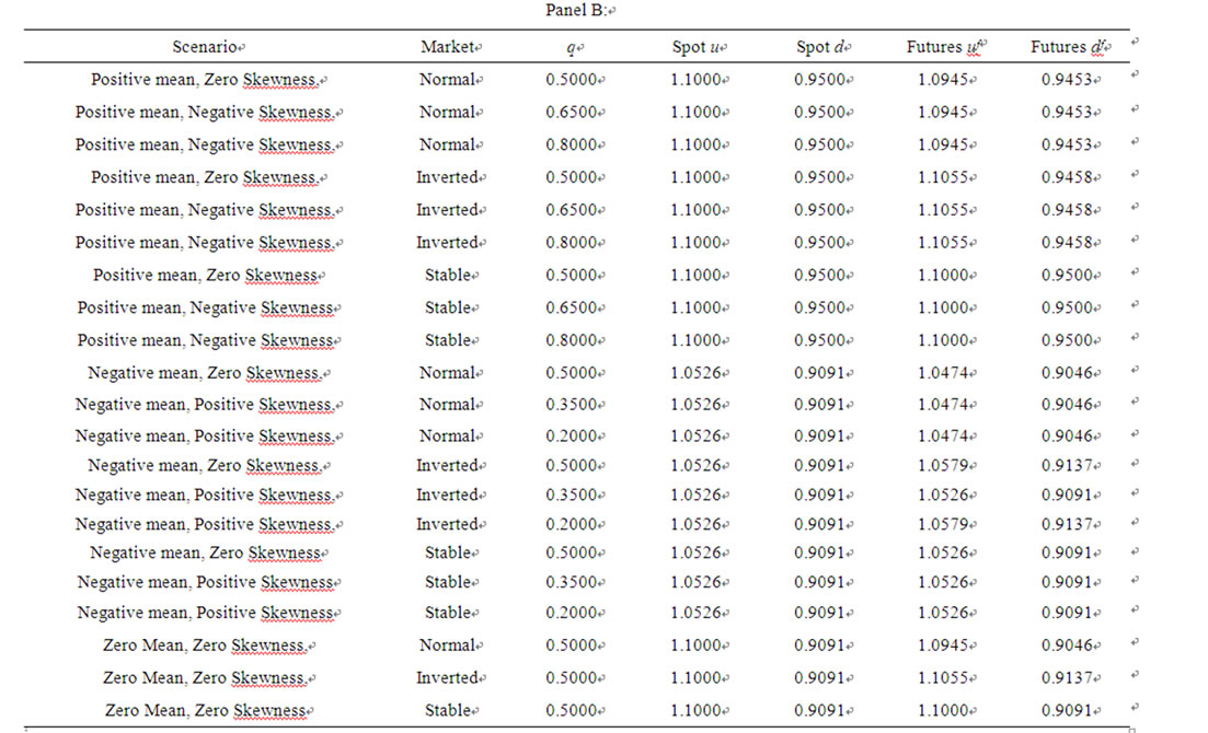
In this market, u > uf and d > df. On the other hand, if R < ψ, then the futures market is inverted with the futures price less than the spot. In this market, uf > u and df > d. Finally, if the net carry cost is zero, then R = ψ and the futures market is neutral; in this market, the futures up and down parameters will be equal to the spot up and down parameters, that is, uf = u and df = d. The relations between the parameters are illustrated in Table 1. The table shows the futures and spot up and down parameters calculated for a number of scenarios: positive mean and negative skewness cases (increasing price case) for normal, inverted, and neutral futures market; negative mean and positive skewness cases (decreasing price case) for normal, inverted, and neutral futures market; and zero mean and skewness case (stable price case) for normal, inverted, and neutral futures market. Panel A in the table shows the inputs for each scenario and Panel B gives the corresponding parameters.
3. Binomial Futures Options Pricing Model
3.1. Decreasing Exchange-Rate Case
Several empirical studies have shown that periods of increasing security prices are often characterized by a positive mean and significant negative skewness in the security price’s logarithmic return. As an example of a decreasing price scenario, suppose the current US dollar/British pound exchange rate is S0 = $1.60/BP, and there is a market expectation of a dollar appreciation over the next year such that the expected distribution of logarithmic returns for the exchange rate has the following annualized mean, variance, and skewness: μS = −0.17597, VS = 0.019555, and δs = 0.0008602. Given these empirical moment values, consider the pricing of call and put options on a British pound (BP) futures contract each with X = $1.60/BP and a time to expiration of 270 days, using a three-period binomial model. In pricing the options, assume the following:
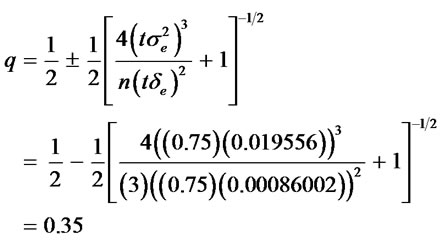
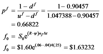
1) The spot $/BP exchange rate at time 0 is E0 = $1.60/BP 2) The annual risk-free rate paid on US dollars is R = 0.06 3) The annual risk-free rate paid on British pounds is ψ = 0.04 4) The futures contract on the BP expires in one year 5) Carrying-cost model holds 6) Options on the BP futures options expire in 270 days 7) 360-day year The length of the binomial period in years is ∆t = t/n = (270/360)/3 = 0.25, with the call and put options expiring in (noption)∆t = (3) (0.25) = 0.75 years, and the BP futures expiring in nf ∆t = (4) (0.75) = 1 year. The up and down parameters for the spot rate are u = 1.052636 and d = 0.9091, the up and down parameters for the futures contract are uf = 1.047388 and df = 0.90457, q = 0.35, the risk-neutral probability is pf = 0.66822, and the equilibrium futures price is $1.63232/BP:
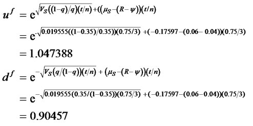
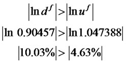
The negative mean and positive skewness in this case yield uf, df, and q values that reflect a decreasing exchange-rate scenario in which the proportional decrease in the futures rate each period is 10.03%, exceeding in absolute value the proportional increase of 4.63%, and the probability of the decrease in each quarterly period (∆t = 0.25) is 1− q = 0.65:
The binomial tree for the underlying spot $/BP exchange rate, BP futures contract, European and American futures calls, and European and American futures puts are shown in Exhibit 1. In the three-period option case, the binomial model prices the European futures call at $0.0857 and the European futures put at $0.0553. As shown in the exhibit, there is an early exercise advantage for the American futures call at the upper node in period 2, and an early exercise advantage for the American futures put at the lower node in period 2. As a result, both the American futures put and call options are price slightly higher than their European counterparts.
If the up and down parameters are not adjusted for skewness, then q = 0.5 and the skewness-adjusted equations for the up and down parameters for the spot and futures simplify to the CRR/RB formulas:
In this example, the up and down parameters for the spot rate would be u = 1.026268 and d = 0.892335, the up and down parameters on the futures contract would be uf = 1.021149 and df = 0.887884, and the risk-neutral probability would be pf = 0.8412978. In this case, in which skewness is assumed to exist but is excluded in the estimates of the up and down parameters the binomial model prices the European call at $0.0786, 8.28% less than the skewness-adjusted model, and the European put at $0.0477, 13.74% less than the skewness model. Additionally, there would not be an early exercise advantage
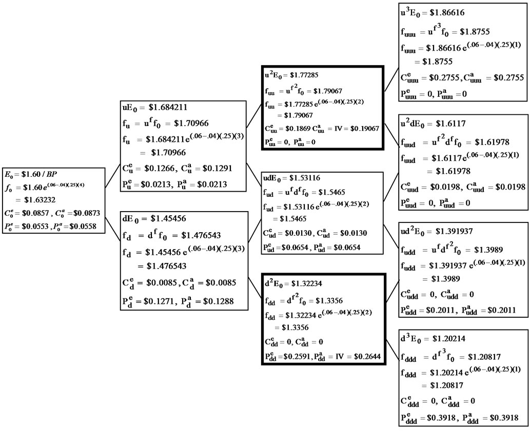
Exhibit 1. Binomial call and put values under decreasing exchange rate case: skewness model.
for the American futures call and there would be only one early exercise advantage for the American futures put. As a result, the American futures put option is priced slightly higher than its European counterpart.
3.2. Increasing Exchange Rate Case
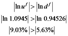
Periods of increasing security prices are often characterized by a positive mean and negative skewness in the security price’s logarithmic return. To illustrate option pricing under this scenario, suppose the market expects the $/BP exchange rate to increase over the next year such that the expected distribution of the exchange rate’s logarithmic return has the following estimated annualized moments: μS = 0.17597, VS = 0.019555, and δS = −0.0008602. In this increasing exchange rate case, the up and down parameters for the spot rate are u = 1.10 and d = 0.95, the up and down parameters on the futures contract are uf = 1.0945 and df = 0.94526, q = 0.65, and the risk-neutral probability is pf = 0.36675. The positive mean and negative skewness yield uf, df, and q values that reflect an increasing exchange-rate period in which the proportional increase in the futures rate each period is 9.03%, exceeding in absolute value the proportional decrease of 5.63%, and the probability of an increase in each quarterly period (∆t = 0.25) is q = 0.65:
In a three-period option case, the binomial model for the increasing case would price the European futures call at $0.0862 and the European futures put at $0.0553. The American futures put and call options are priced slightly higher than the European option, given early exercise advantages for both the call and put options.
If the up and down parameters for this increasing case were not adjusted for skewness, then q would be equal to 0.5, and the up and down parameters for the spot rate would be u = 1.120667 and d = 0.974407, the up and down parameters on the futures contract would be uf = 1.115078 and df = 0.969547, and the risk-neutral probability would be pf = 0.20925. In this case in which skewness is assumed to exist but is excluded in the estimates of the up and down parameters, the binomial model prices the European call at $0.084, 2.55% less than the skewness-adjusted model, and the European put at $0.0531, 3.98% less than the skewness model.
4. Properties of the Skewness Model
In the case of spot options, the existence of skewness affects the relative contribution of the mean to the values of the up and down parameters and the asymptotic properties, with the skewness-adjusted up and down parameters having different asymptotic properties than the CRR/RB parameters. In the case of futures options, these same properties also hold. In addition, with futures options, the impact skewness has on elevating the importance of the mean depends on the carrying cost value (R − ψ) and whether the futures market is normal, inverted or neutral.
4.1. Relative Importance of the Mean Term
In the case of a positive mean, the mean becomes more important in determining the value of the spot up parameter value, the greater the negative skewness (or equivalently the more q exceeds 0.5). Similarly, for futures options, the µ − (R − ψ) term becomes more important in determining the futures up parameter value (uf), the greater the negative skewness. By contrast, in the case of a negative mean, the mean becomes more important in determining the value of d, and the µ − (R − ψ) term becomes more important in determining the value of the futures down parameter (df), the greater the positive skewness (or equivalently the more 1 − q exceeds 0.5).
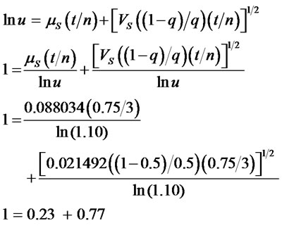
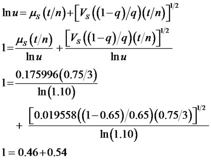
To see the impact skewness has on increasing the importance of the mean for spot options and the µ − (R − ψ) term for futures options, consider the previous threeperiod increasing exchange rate case in which u = 1.10 and d = 0.95 for the spot exchange rate. If skewness were zero, then q would be equal to 0.5, the expected quarterly mean would be equal to 0.020084 (=[(0.5)ln(1.10) + (0.5)ln(0.95)]) and the annualized mean would be 0.088034. The quarterly variance would be equal to 0.0053731 (= 0.5[ln (1.10) − 0.020084]2 + 0.5[ln (0.95) − 0.020084]2), and the annualized variance would be 0.021493. If these were the actual empirical values of µS and VS, then ln(u) would be equal to 0.0953 (u = 1.10), and the mean would contribute 23% to the value of u and the variance would contribute 77% to the value of u:
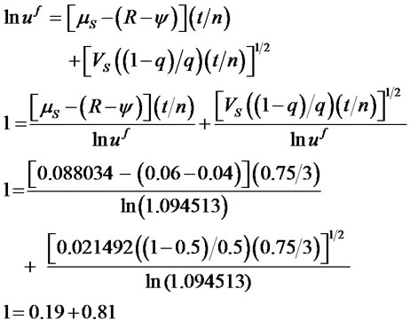
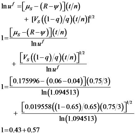
For the futures option, the ln(uf) would be equal to 0.0903095 (uf = 1.094513) given the net cost of carry of 0.02 (=R – ψ = 0.06 − 0.04). The mean minus the net cost of carry (R – ψ) would, in turn, contribute 19% to the value of uf and the variance would contribute 81% to the value of uf:
If negative skewness were present such that q = 0.65, then the quarterly mean would be equal 0.044 (= [(0.65) ln(1.10) + (0.35) ln(0.95)]) and the annualized mean would be 0.176. The quarterly variance would, in turn, be equal to 0.0389986 (= 0.65 [ln(1.10) − 0.044]2 + 0.35 [ln(0.95) − 0.044]2) and the annualized variance would be 0.019558. Given the mean and variance values and a q = 0.65, the implied skewness would be δ = −0.0008602. If these were the actual empirical values of mean, variance, and skewness, then ln(u) would be equal to the nonskewed value of 0.0953 (u = 1.10), but with q = 0.65, the contribution of the mean to the value of u would be 46% and the contribution of the variance to the value of u would be 54%:
For the futures options, the ln(uf) would likewise be equal to its non-skewed value of 0.0903095 (uf = 1.094513), but the contribution of the mean and the net cost of carry (R – ψ) term to the value of uf would be 43%, and the contribution of the variance to the value of uf would be 57%:
Thus, in the case of a positive mean, negative skewness increases the relative importance of the mean on the up parameters for the spot and futures rates1.
By contrast, in the case of a positive mean, the mean term has an opposite directional impact on d and df than the variance term, with its negative impact increasing the greater the negative skewness (or equivalently the more q exceeds 0.5). For example, in the no skewness case for the futures option, ln(df) is equal to −0.056292 (df = 0.945262). In this case, the µ − (R − ψ) term would contribute −30% to the value of df and the variance term would contribute 130% to the value of df. In the skewness case, the µ − (R − ψ) term would contribute −69% to the value of df, whereas the variance would contribute 169% to the value of df:
Just the opposite relationships hold in the case of a negative mean with positive skewness. Specifically for a negative mean, the mean becomes more important in determining d and df the greater the positive skewness, whereas the mean term has an opposite directional impact on u and uf than the variance term, with its negative impact on the up parameter increasing the greater the positive skewness. Table 2 summarizes the relative contributions of the mean and variance terms to the spot and futures up and down parameters for the decreasing exchange-rate case and other scenarios with different levels of skewness and different futures markets. Panel A details the relative contributions for the spot and Panel B details the contributions for the futures.
4.2. Asymptotic Properties
In the CRR/RB model, as the number of subperiods (n)
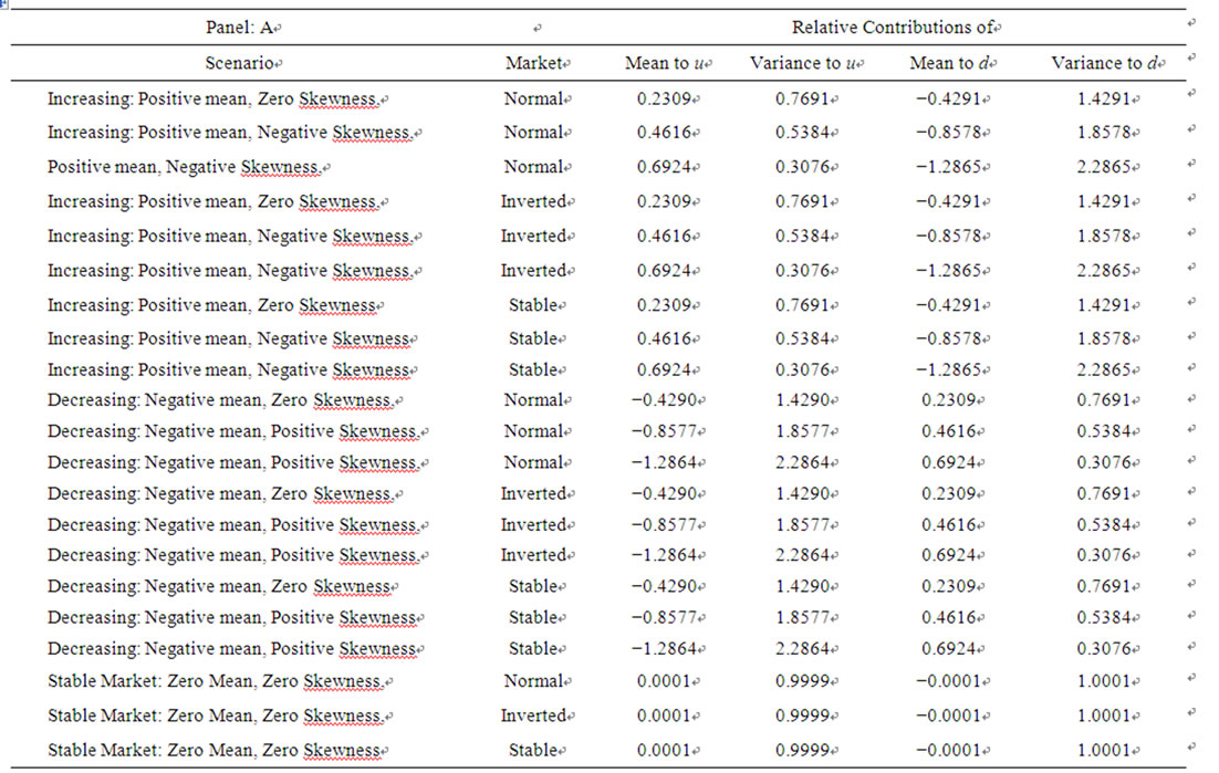
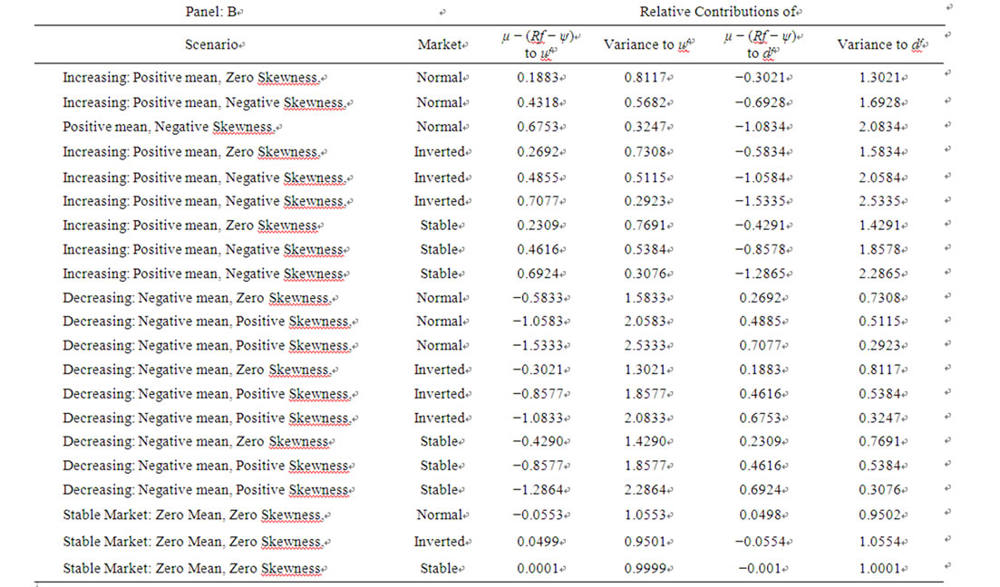
Table 2. (a) Relative contributions of the mean and variance terms to up and down parameters; (b) Relative contributions of the mean and variance terms to up and down parameters.
increases, the mean term in the exponent for spot options and the µ − (R − ψ) term for futures options go to zero faster than the square root term. Thus for large n, the CRR/RB model depends only on the volatility. Moreover, with σS = σf, the up and down parameters for the futures are equal to the spot, regardless of whether the futures market is normal or inverted:
Using theses up and down parameters, the BOPM for futures options converges to the seminal Black futures option model [13] as n gets large.
The skewness-adjusted up and down parameters, though, do not have the same asymptotic properties as the CRR/ RB parameters. In the skewness model, equation (20) for uf includes a(1 − q)/q term, and equation (21) for df includes a q/(1 − q) term, both of which change the order of magnitude as n gets large. Specifically, for the case of negative skewness, the (1 − q)/q term can be rewritten as:
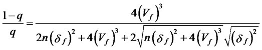 (22)
(22)
The expression (1 − q)/q in equation (22), in turn, is the same order of magnitude as 1/n. This can be seen by observing that the term [(1 − q)/q]/[1/n] approaches the constant 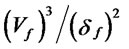 as n gets large. That is:
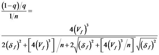 (23)
(23)
and in the limit:
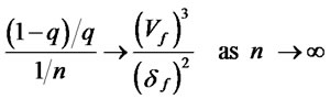 (24)
(24)
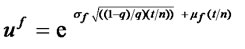
With (1 − q)/q having the same order of magnitude as 1/n, the term [(1 − q)/q*Vf/n]1/2 in Equation (13) ap- proaches a constant multiplied by [Vf]1/2/n, as n gets large. As a result, for the case of large n, the first term in the exponent in equation (13) approximates a constant divided by n, which is in the same form as the second term, μf/n = (μS − (R − ψ))/n.
Consequently, both terms in the exponent of equation (13) for uf contribute equally, even when n is large. Thus, as n gets large, uf depends not only on the variance and skewness, but also on the mean, risk-free rate, and asset yield. By contrast, equation (14) for df is defined in terms of q/(1 − q). In this case, as n gets large, the variance term in the exponent for df approaches the constant δf/Vf and the μf/n term approaches zero. Thus, for the case of negative skewness with a large n, df depends on the variance and skewness, but not on the mean, risk-free rate and dividend yield, whereas uf depends on all three parameters. Just the opposite asymptotic relationships occur when skewness is positive. In this case, the mean, variance, skewness, risk-free rate, and dividend yield determine df (even when n is large), whereas just the variance and skewness determine uf.
Note, similar asymptotic relations also hold for the spot up and down parameters, with the spot and futures asymptotic relations being equivalent when the net cost of carry is zero (R − ψ = 0).
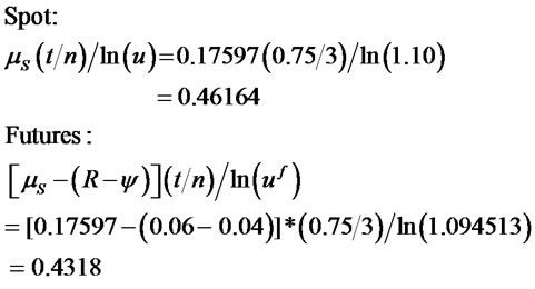
To illustrate the relative importance of the mean for the case of large n, consider the preceding increasing exchange-rate case (option expiring in 0.75 year, R = 0.06 and ψ = 0.04) where the estimated annualized mean, variance, and skewness were μS = 0.17597, VS = 0.0019555, and δS = −0.0008602. If we subdivide the option period (t = 0.75) into 3 subperiods (n = 3), then for the spot exchange rate the mean term would contribute 46.164% to the value of u and the variance term would contribute 53.836% to the value of u; for the futures, the µ − (R − ψ) term would contribute 43.18% to the value of uf and the variance term would contribute 56.82% to the value of uf:
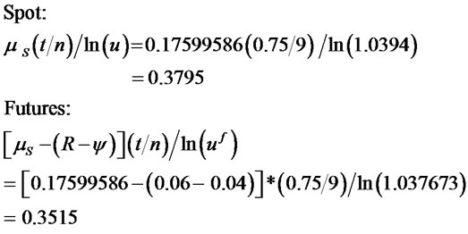
If we subdivide the option period into nine monthly subperiods (n = 9; t/n = 0.75/9 = 0.08333; u = 1.03940, d = 0.9481; uf = 1.037673, df = 0.9465), the mean term would contribute 37.95% and the variance term would contribute 62.05% for the spot rate, and for the futures, the mean term would contribute 35.15% and the variance term would contribute 64.85%:
For larger n, the contribution of the mean is approximately the same: when n = 39 (weekly periods; t/n = 0.75/39 = 0.01923), the relative contribution of the mean would be 31.59% for the spot rate and 29.04% for the futures; when n = 270 (daily; t/n = 0.75/270 = 0.0028), the contributions would be 28.91% for the spot and 26.49% for the futures; when n = 1000, the contributions would be 28.51% and 26.11% for the spot and futures, respecttively; when n = 1000000, the contributions would be 28.35% and 25.97%.
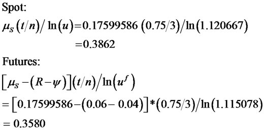
By contrast, if skewness were zero (the CRR/RB model with µS = 0.17597, VS = 0.019558, and δS = 0), the relative contributions of the mean term for the spot rate and futures would be 38.62% and 35.80% for n = 3 ((n = 3; t/n = 0.75/9 = 0.08333; u = 1.120667, d = 0.974407; uf = 1.115078, df = 0.969547):
When n = 9, the mean contribution for the spot and futures, respectively, would be 26.64% and 24.36%; when n = 39, 14.86% and 14.40%; when n = 270, 6.22% and 5.55%; when n = 1000, 3.33% and 2.96%; and when n = 1000000, 0.1% and 0.1%.
Figure 1 shows graphically the relationship between the number of subperiods and the mean’s contribution to the up parameter for the skewness-adjusted increasing exchange-rate case.
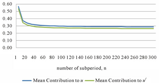
The graph in Figure 1 highlights the asymptotic relation, showing that as n increases, the mean’s contribution to both the sopt and futures up parameters decreases asymptotically with the asymptote occurring at approximately n* = 30 where the minimum mean contribution is 30%2. Figure 2 summarizes the relationship between the number of subperiods and the mean’s contribution to the up and down parameters for the CRR/RB case in which skewness is zero.
Figure 2. Mean contribution to u and uf, μS = 0.175996, VS = 0.019558, δS = 0.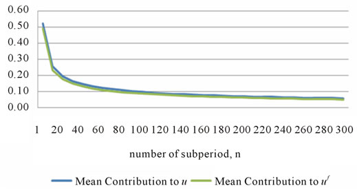
Figure 2, in turn, shows a similar asymptotic relation between the mean’s contribution and n for the CRR/RB model as the skewness case, but with the minimum mean contribution being close to zero.
Figure 3. Mean contribution to d and df, μS = –0.17597, VS = 0.019555, δS = 0.00086019.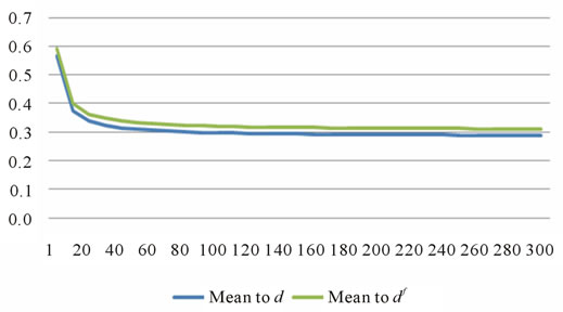
Figure 3 shows graphically the relationship between the number of subperiods and the mean’s contribution to the down parameters for the skewness-adjusted decreasing exchange-rate case characterized by a negative mean and positive skewness: µS = −0.17597; VS = 0.019555; δS = 0.0008602. The graph highlights the asymptotic relation, showing that as n increases, the mean’s contribution to the down parameters decreases asymptotically with the asymptote occurring at approximately n* = 30 where the minimum mean contribution is 30%.
Figure 4. Mean contribution to d and df, μS = –0.17597, VS = 0.019555, δS = 0.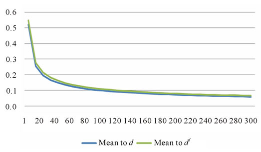
Figure 4 shows a similar asymptotic relation between the mean’s contribution to the down parameter and n for the CRR/RB case, but with the minimum contribution being close to zero.
5. Differences in Futures Option Prices between the CRR/RB Model and the Skewness-Adjusted Model
Values for European futures call options on the British pound obtained using the skewness-adjusted model and the CRR/RB Model are presented in Table 3, and values for the European futures put options on the British pound are shown in Table 4. The call and put futures options each have exercise prices of $1.60/BP and expire in 0.75 years, and the British pound futures contract expires in one year, with the futures price assumed to be equal to its carrying-coat value. The binomial model used for pricing is subdivided into 60 periods of length 6 days. The tables show three futures markets: a normal futures market where the annualized risk-free rate is assumed to be 6% on US dollars and 4% on British pounds, an inverted market where the dollar rate is 4% and British pound rate is 6%, and a neutral market where each rate is equal to 6%. Finally, the tables show two exchange-rate scenarios:
1)
An increasing exchange-rate case characterized by a positive mean and a negative skewness: μS = 0.17599586, VS = 0.019558, δS = −0.000860192.2)
A decreasing exchange-rate case characterized by a negative mean and a positive skewness: μS = 0.17599586, VS = 0.019558, δS = −0.A comparison of the futures option values obtained using the skewness-adjusted model with the CRR/RB model illustrates th
e pricing differences that occur under increasing or decreasing exchange-rate cases characterized by skewness. In general, for both scenarios, the CRR/RB model prices the American and European futures call and the American and European futures puts less than the skewness model, with the greatest pricing differences occurring for out-of-the-money options. Specifically, the si-mulations show underpricing of the CRR/RB model, ranging from approximately 5% for in-the-money options to approximately 35% for out-of-the-money options. For the futures call option, in both the increasing and decreasing cases, the CRR/RB model underprices more for the inverted futures market case (range 30.56% - 10.11% (increasing); 39.43% - 5.93% (decreasing)) than the normal futures market case (21.59% - 5.63% (increasing); 34.79% - 4.10% (decreasing)). For puts, the CRR/RB model underprices more for the normal market case (range 5.05% - 38.36% (increasing); 9.14% - 30.80% (decreasing)) than the inverted market case (4.67% - 33.06% (increasing); 4.85% - 21.25% (decreasing))3.
Finally, Table 5 compares futures call and put prices with corresponding spot call and put prices for normal, inverted, and neutral futures market under a stable exchange-rate scenario in which the mean and skewness are zero. As shown, with zero skewness, the skewness model and the CRR/RB model for spot and futures options are the same. The simulations, in turn, also show that this is the only case in which European futures and spot options are equal.
6. Conclusions
A subtle feature of the B-S model and the BOPM for large n is that these models depend only on the variance. The mean is not important in determining the value of spot options, and the mean and net carry cost are not important for futures options. This feature is a consequence of the assumption that the logarithmic return of the underlying security is normally distributed. In this paper, we show that in cases where skewness exists, the skewness-adjusted up and down parameters for spot options depend more on the mean than non-skewness-adjusted parameters, and that the skewness-adjusted up and down parameters for futures options depend more on the µ − (R − ψ) term than non-skewness-adjusted parameters. Furthermore, the skewness-adjusted up and down parameters also have different asymptotic properties such that for large n, the mean for spot prices and the µ − (R − ψ) term for futures maintain their relative importance.
Thus, the presence of skewness serves to augment the relative importance of the mean for spot options and the µ − (R − ψ) term for futures options. Using simulations, we show that when there is an expected increasing price trend characterized by a positive logarithmic mean and
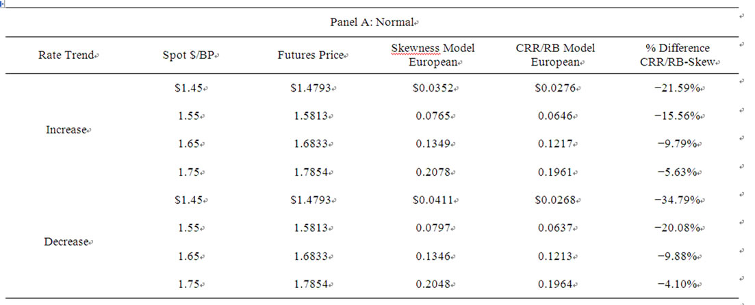
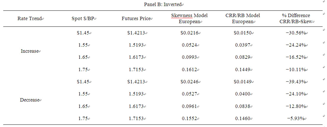
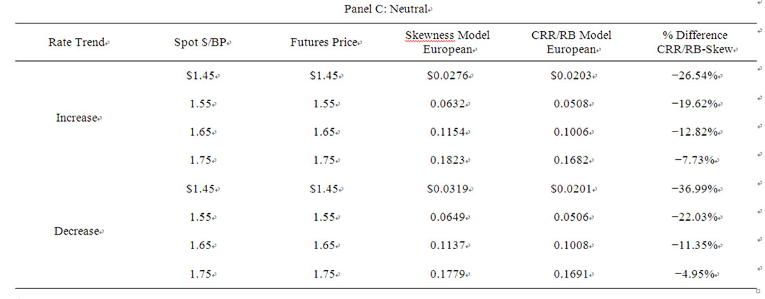
Table 3. Comparison of skewness-adjusted futures option model with crr/rb model for normal, inverted and neutral futures markets and increasing and decreasing exchange-rate trends: european futures call options.
negative skewness or an expected decreasing price trend characterized by a negative logarithmic mean and positive skewness, the CRR/RB model for large n when compared to the skewness-adjusted futures options model underprices futures options between 4% and 30%, with the larger underpricing occurring for out-of-the money options.
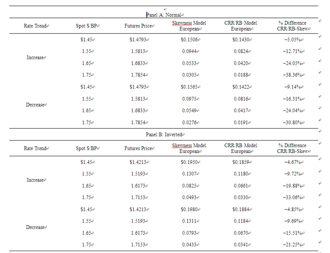
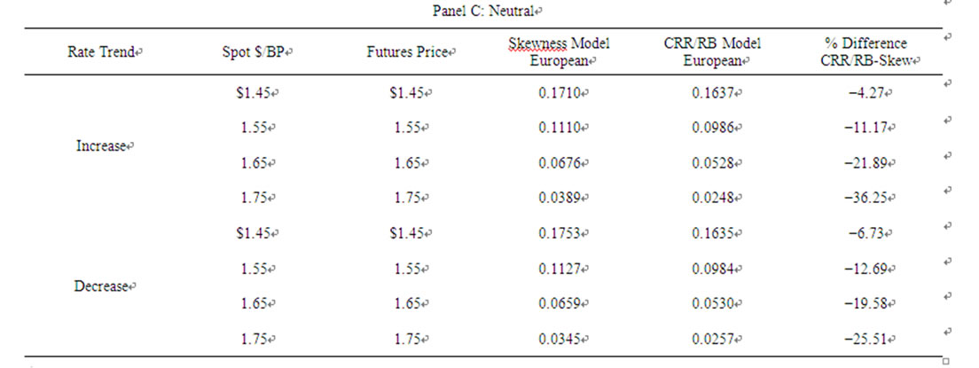
Table 4. Comparison of skewness-adjusted futures option model with crr/rb model for normal, inverted and neutral futures markets and increasing and decreasing exchange-rate trends: european futures put options.
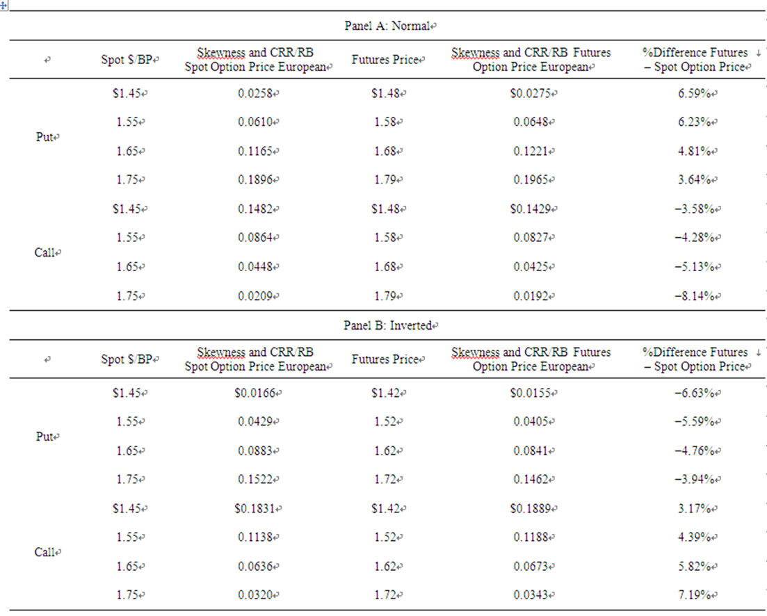
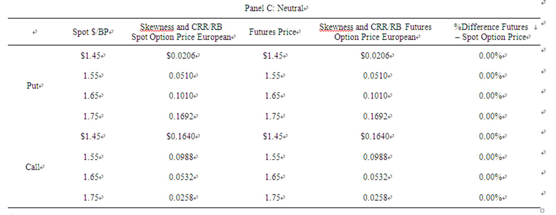
Table5. Comparison of european spot and future option prices for normal, inverted and neutral futures markets and a stable exchange-rate market.
Moreover, with the relative contribution of the mean and carrying cost values for a large number of subperiods being at least 30% for one of the up or down parameters in the skewness model and minimal in the CRR/RB, the underpricing can be explained by the change in asymptotic properties resulting from skewness that elevate the importance of the mean and carrying cost parameters. Finally, it should be noted that the BOPM for futures options converges to the seminal Black futures option model as n gets large given a normal distribution for the logarithmic return. The Black futures model, in turn, differs from the B-S Merton model used for pricing spot options by the exclusion of the risk-free rate and the asset yield in the equations for d1 and d2. This difference, though, only holds given the assumption of normality. If skewness exists, then the risk-free rate and asset yield, as well as the mean, become important in pricing futures options for the discrete binomial model, as well as the Black futures option model.
REFERENCES
- R. S. Johnson, J. E. Pawlukiewicz and J. Mehta, “Binomial Option Pricing with Skewed Asset Returns,” Review of Quantitative Finance and Accounting, Vol. 9, No. 1, 1997, pp. 89-101. doi:10.1023/A:1008283011490
- F. Black and M. Scholes, “The Pricing of Options and Corporate Liabilities,” Journal of Political Economy, Vol. 81, No. 3, 1973, pp. 637-659. doi:10.1086/260062
- R. S. Johnson, R. A. Zuber and J. M. Gandar, “Binomial pricing of Fixed-Income Securities for Increasing and Decreasing Interest Rate Cases,” Applied Financial Economics, Vol. 16, No. 14, 2006, pp. 1029-1046. doi:10.1080/09603100500426473
- R. S. Johnson, R. A. Zuber and J. M. Gandar, “Pricing Stock Options under Expected Increasing and Decreasing Price Cases,” Quarterly Journal of Business and Economics, Vol. 46, No. 4, 2007, pp. 63-90.
- E. M. Stein and J. C. Stein, “Stock Price Distributions with Stochastic Volatility: An Analytical Approach,” Review of Financial Studies, Vol. 4, No. 4, 1991, pp. 727-752. doi:10.1093/rfs/4.4.727
- J. B. Wiggins, “Option Values under Stochastic Volatility: Theory and Empirical Estimates,” Journal of Financial Economics, Vol. 19, No. 2, 1987, pp. 351-372. doi:10.1016/0304-405X(87)90009-2
- S. L. Heston, “A Closed Form Solution for Options and Stochastic Volatility with Applications to Bond and Currency Options,” Review of Financial Studies, Vol. 6, No. 2, 1993, pp. 327-344. doi:10.1093/rfs/6.2.327
- R. Jarrow and A. Rudd, “Approximate Option Valuation for Arbitrary Stochastic Processes,” Journal of Financial Economics, Vol. 10, No. 3, 1982, pp. 347-369. doi:10.1016/0304-405X(82)90007-1
- C. J. Corrado and T. Su, “Skewness and Kurtosis in S&P 500 Index Returns Implied by Option Prices,” The Journal of Financial Research, Vol. 19, No. 2, 1996, pp. 175- 192.
- A. Câmara and S. Chung, “Option Pricing for the Transformed-Binomial Class,” The Journal of Futures Markets, 2006, Vol. 26, No. 8, pp. 759-787. doi:10.1002/fut.20218
- J. C. Cox, S. A. Ross and M. Rubinstein, “Option Pricing: A Simplified Approach,” Journal of Financial Economics, Vol. 7, No. 3, 1979, pp. 229-263. doi:10.1016/0304-405X(79)90015-1
- R. J. Rendleman and B. J. Bartter, “Two-State Option Pricing,” Journal of Finance, Vol. 34, No. 5, 1979, pp. 1093- 1110. doi:10.2307/2327237
- F. Black, “The Pricing of Commodity Contracts,” Journal of Financial Economics, Vol. 3, No. 1-2, 1976, pp. 167-179. doi:10.1016/0304-405X(76)90024-6
NOTES
1
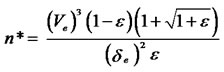
Note that in this case, µ > (R − ψ) and the futures market is normal (R – ψ > 0) with the futures price exceeding the spot price. As a result, negative skewness increases the mean’s impact on the up parameter (46%) for the spot option more than the up parameter for the futures option (43%). In contrast, if the market were inverted (R – ψ < 0), then negative skewness would have decreased the impact of the mean on the futures up parameter more than the spot parameter.2It should be noted that since all the parameters contribute to either lnu or lnd as n gets large, the n value in which the skewness-adjusted model approaches a continuous one depends on the relative values of µS, VS, and δS. For the case of δS < 0, the term (1 − q)/q approaches a constant divided by n in the limit. The critical value, n*, can therefore be found by solving for the n that makes (1 − q)/q (Equation (20)) equal to a large proportion (e.g., 0.99) of the limit (Equation (22)). Defining the proportion as 1 − ε, where ε is equal to the proportion of error (e.g., ε = 0.01), the n* that is equal to 1 − ε of the limit is:
3The pricing differences between the CRR/RB model and the skewness model are consistent with the aforementioned empirical studies of Stein and Stein [4], Wiggins [5], and Heston [6] who demonstrate that when skewness exists, the B-S model consistently underprices options. Also, as expected, there were no significant difference in the prices for the European call and put options obtained using the Black futures option model (not shown) and the 60-period CRR/RB binomial prices shown in Table 5.