Open Journal of Statistics
Vol.05 No.06(2015), Article ID:60830,14 pages
10.4236/ojs.2015.56062
Computational Method for Extracting and Modeling Periodicities in Time Series
Eduardo González-Rodríguez1, Héctor Villalobos2, Víctor Manuel Gómez-Muñoz2, Alejandro Ramos-Rodríguez1
1Oceanografía Tropical, CICESE Unidad La Paz, La Paz, Mexico
2Instituto Politecnico Nacional-CICIMAR, La Paz, B.C.S, Mexico
Email: egonzale@cicese.mx
Copyright © 2015 by authors and Scientific Research Publishing Inc.
This work is licensed under the Creative Commons Attribution-NonCommercial International License (CC BY-NC).
http://creativecommons.org/licenses/by-nc/4.0/


Received 28 July 2015; accepted 27 October 2015; published 30 October 2015
ABSTRACT
Periodicity is common in natural processes, however, extraction tools are typically difficult and cumbersome to use. Here we report a computational method developed in MATLAB through a function called Periods with the aim to find the main harmonic components of time series data. This function is designed to obtain the period, amplitude and lag phase of the main harmonic components in a time series (Periods and lag phase components can be related to climate, social or economic events). It is based on methods of periodic regression with cyclic descent and includes statistical significance testing. The proposed method is very easy to use. Furthermore, it does not require full understanding of time series theory, nor require many inputs from the user. However, it is sufficiently flexible to undertake more complex tasks such as forecasting. Additionally, based on previous knowledge, specific periods can be included or excluded easily. The output results are organized into two groups. One contains the parameters of the adjusted model and their F statistics. The other consists of the harmonic parameters that best fit the original series according to their importance and the summarized statistics of the comparisons between successive models in the cyclic descent process. Periods is tested with both, simulated and actual sunspot and Multivariate ENSO Index data to show its performance and accuracy.
Keywords:
Time Series, Cyclic Descent, Harmonic, Periodicity, Forecasting, Sunspot, Multivariate ENSO Index

1. Introduction
Periodic or cyclic phenomena are characteristic of many different kinds of data [1] . In natural sciences, in particular, the periodic behavior of biological events is of interest for many reasons, e.g. to explain the fluctua- tions in abundance of animals or plants. Sardine abundance, for instance, shows cyclic fluctuations of varying frequencies that can be related to environmental events of short term variability like El Niño Southern Oscillation (~5 - 8 years), low (~20 years) and very low frequency (~60 years) ocean climate variations [2] .
The task of finding periodicities in data is typically made using signal processing techniques or spectral analysis, but it requires a solid mathematical background. In recent years, there has been a great interest in developing alternatives like the matching pursuit algorithm [3] , which consists of the decomposition of a time series into several waves or dictionaries (i.e. wavelets, Gabor dictionaries and many others). However, this method and other closely related ones require the parametrization waveform of the chosen dictionary [4] to be supplied by the user. In many cases, this may not be easy to do specially for non-mathematical specialists like biologists, ecologists, economists, financial analysts or social researchers.
In contrast, in this paper we develop a computer method through a MATLAB function called Periods, which is based on classical Fourier analysis, whose underlying math is easy to understand and does not require a deep knowledge of the Fourier theory. Also, such function it is able to identify all of the significant cyclic com- ponents and the linear trend (if present) in a time series and, if desired, to make predictions outside of the observed values.
We tested the performance of the Periods function with a time series simulated with known Periods and also with the well known yearly sunspot series and MEI (Multivariate El Niño Southern Oscillation Index) series. The results were compared to values reported in the literature to evaluate accuracy.
2. Methodology
For the purpose of this paper we define a time series as a sequence of data points , measured at successive times (t) uniformly spaced (regular time series). Besides periodic variations
 , a time series may also show a linear trend
 (1)
(1)
In Equation (1),  represents a random error component. If the presence of a linear trend is suspected, the linear regression of
  on t should be done and the fitted series removed from the original series to isolate the cyclic component
 (2)
(2)
The cyclic component can be represented by a cosine wave [5] [6]
 (3)
(3)
This function is defined by the length of the cycle (period p), one-half the range from the minimal to the maximal response (semi-amplitude A, hereafter referred to as amplitude for simplicity) and the angular point in time during the cycle when the response is a maximum (phase angle ). The mean response over a number of complete periods is given by
  [5] . To simplify the model the mean is subtracted from the time series so
 .
.
When the period is known, the estimation of amplitude and phase angle can be done by regression, which in this context is referred as periodic regression [5] . This method involves rewriting Equation (3) in its linear form
 (4)
(4)
here  is the angular frequency, and the parameters
  and
and  are unknowns, which can be estimated by multiple regression. They relate to amplitude (A) and phase angle (
 , from now on called phase for simplicity) by the following equations
 (5)
(5)
 (6)
(6)
when .
.
From the following equation
 (7)
(7)
the graphical lag from the origin (L) can be calculated as
 (8)
(8)
When there are several periodicities in the data, the model will consist of a sum of sinusoidal functions [6] [7] , each one of them defined by their own parameters ( ,
, and
and )
)
 (9)
(9)
2.1. Periodic Regression
The proposed procedure for finding the period and corresponding amplitude and phase angle for each harmonic that best fits , involves sequentially testing every value in a given set of periods, and estimating the model parameters (
 and
and ) from equation 4 while testing which model best fits the data.
For the set of periods to test, a reasonable initial value (ip) is three (in the same units of time as the original data) while the final value (fp) will depend on the length of the time series (n).
2.2. Optimum Period
In order to select the optimum period (op) in the tested sequence, an analytical and graphical criterion is introduced. This criterion is called the maximal reciprocal of residual sum of squares (MRRSS). Analytically, the objective consists of adjusting the parameters of a model function to best fit the data set based on the residual sum of squares (RSS); graphically, RSS values close to zero are amplified and represent peaks denoting the optimum period. The mathematical representation is as follows:
 (10)
(10)
where  is defined by
 (11)
(11)
and where  is the fitted series corresponding to period p. Let op be the optimal period that satisfies Equation (10).
2.3. Cyclic Descent
Once the first op has been found, the fitted series  becomes
  and is subtracted from
  producing a residual series
 (12)
(12)
The periodic regression will then be applied sequentially to the  series to identify all the op according to the MRRSS criterion for each one of the harmonics i in the time series, hence Equation (12) can be rewritten as follows:
 (13)
(13)
where  is the fitted series for the i-th optimum period. This process of cyclic descent [1] is repeated until the last significant harmonic m is found. As this process is carried out, simultaneously
  are summed to
 (14)
(14)
To determine if the addition of the new harmonic component is statistically significant (continuing the search of periods), we use a likelihood ratio test [8]
 (15)
(15)
where  and
and  are the residual sum of squares of the models including respectively harmonic
  and i;
  and
and  are the corresponding number of parameters of the models and n is the length of the time series. The statistic
  has an F distribution with
  and
and  degrees of freedom.
Once the last significant harmonic is found, in order to determine the best estimates of the amplitude and phase for each one, a final model including all the harmonics is fitted by multiple regression
 (16)
(16)
In this equation,  and
and  are the linear regression coefficients when a linear trend is assumed, otherwise both parameters equal zero.
 ,
,  and
and  are the corresponding parameters of the i-th harmonic. Both
  and
and  are finally used to calculate the amplitudes and phase angles with Equations (5) and (6).
3. Computational Method
This section describes the computational method developed trough the Periods function, which incorporates the above described methodology and other additional steps.
The complete set of arguments and default values of the Periods function in MATLAB1 is:
Periods (x, varargin)
where varargin represents the rest of the optional arguments, detailed below:
・ x: Time series
A vector containing the time series to be analyzed. Any variable name can be used, not restricted to x.
The next arguments are optional, with default values if not provided. They allow the user to control and fine tune the performance of the function and the degree of detail of the results.
・ t: Time vector
Must be a monotonically increasing vector of the same length of x. Usually data is collected in regular intervals in time. However, in long series this is not always the case. For example, the MEI series used in the results section, the data is arranged on a “monthly” basis, which is not a regular time unit due that a “month” in this series can have 28, 29, 30 or 31 days. In the case of sunspot time series, the time unit should be 365.25, which is the real value in days of a given year. For such reason, it is recommended using the date vector in the format given for the datenum function of MATLAB to obtain a precise time unit. This can have a effect on improving the fit. However, it is user’s decision to experiment and try to evaluate the results.
・ predict: t values for predictions
Integer used when a prediction is desired. If positive a forecast is done, when negative a hindcast is done. Both elements can be supplied indicating prediction in both directions. A time vector can also be provided, in this case a prediction over the vector time will be done. predict values or vector should be in the same units as time vector (t). When used, a new element (Xef) will be added to the output inside Final_Model array.
・ trend: Linear trend (string)
A logical. If TRUE, the linear tendency is calculated and subtracted from the data series, default is FALSE. This option is recommended to be used when the data has a clear tendency.
・ ip: Initial period to test
・ lp: Last period to test
To save computational time two criteria are applied to determine ip and lp. To avoid randomness, ip starts at 3 and lp is restricted to half the length of  (plus one for odd time series), so the harmonic component must be represented at least twice. For example, in a series
  of 1001 data, lp = 501.
・ step: Period step
Is the increment in time for each tested period according to the time unit (derived from t above), the default value is 1 assuming that two successive data values are separated by one unit of time. However, step can take values between 0 and 1. In the previous example the periods to be tested can be 3, 4, 5, …, 501. Changing the default to step = 0.1 the sequence of testing periods to test becomes 3.1, 3.2, 3.3, …, 501. It is important to note that small step consumes more computational time.
・ hn: Harmonics number
Number of harmonics to estimate. Determined by the MRRSS criteria or an integer number supplied by the user.
・ neig: Neighbors
By default, a period identified (op) in a periodic regression will not be considered in a subsequent search unless neig = −1. Other positive integers will cause the function to also exclude neighboring periods:  neig and
  neig in subsequent searches, note that the neighbors are directly related to the step argument.
・ known: Known periods
This option completely overrides the search for periods in cyclic descent. A model with the given known periods is fitted by multiple regression to the x series.
・ include: Include periods
This option allows the user to specify the period(s) to be included in the final fitted model after the search for periods in the cyclic descent has ended.
・ exclude: Exclude periods
The periods given here will be excluded in the periods search.
・ alpha: Significance level, a
The confidence level for the statistical test in the cyclic descent or probability error if the corresponding model fit is rejected. Defaults to alpha = 0.05.
・ rrss: Reciprocal of residual sum of squares (string)
Logical, defaults to FALSE. If TRUE, the periods tested and their corresponding RRSS in every step of the cyclic descent will be provided.
・ plots: Produce plots
A string indicating the desired plots. By default plots = “last”, in which case just the plot with the final fitted model is generated. With plots = “all” the RRSS versus tested periods and the cumulated harmonics fit in every step of the cyclic descent will be plotted in addition to the final fit. When plots = “none” no plot is produced. Can be abbreviated.
Besides the graphical output, the Periods function also outputs a list object with two structure arrays in MATLAB, called Cyclic_Descent and Final_model, they are composed as follows.
Cyclic_Descent: Contains the results of the cyclic descent method and the statistical test in each step:
・ Harmonics: period, amplitude, phase, lag phase, RSS and R2 for every harmonic found;
・ Stats: F statistic, the corresponding degrees of freedom and p-values for the comparison between successive models;
・ RRSS: the periods tested and the corresponding RRSS in every step of the cyclic descent. Only returned if rrss = TRUE.
Final_Model: Contains the final fitted model (Equation (16)) and the corresponding statistical results:
・ Xe: the fitted series;
・ Xef: the predicted time series, only given if the predict argument is used. In this case both the new t values and the corresponding predictions will be provided;
・ Params: parameters for the final model. When trend = TRUE linear trend coefficients ( and
and ) are given, otherwise only the period, amplitude, phase and lag phase for the cyclic components are provided;
・ F_stats: ,
,  , F statistic, the corresponding degrees of freedom and p-value for the final fitted model.
4. Results
4.1. Analysis of a Simulated Time Series
As a first example of the use of the Periods function, a time series (sim, n = 220) comprised by four harmonic components with: periods = 25, 10, 16, 73; amplitudes = 40, 20, 10, 5; phases = 2, 5, 1, 0; ; no trend and 10% of random noise was simulated with Equation (9). The sim time series was analyzed with the defaults producing all the cyclic descent plots.
>> plots = “a”
>> [Final_model, Cyclic_Descent] = Periods (sim, plots)
When running the function, a succession of graphic windows with two panels each appears as the harmonics are found. In the upper panel the RRSS values are plotted against tested periods. op refers to the optimal period found in a given step of the cyclic descent, which corresponds to MRRSS values (Equation (10)) for a given harmonic (the user has the option to output the RRSS used to produce this plot, specifying rrss = TRUE). In the bottom panel, the x series and the fitted model (one harmonic in the first plot, and thereafter the sum of the current with preceding harmonics) are shown, along with the corresponding coefficient of determination . Figure 1 shows these plots arranged side by side in order to simplify the description.
In the left panel the effect on the value of RRSS becomes apparent as harmonics are found and subtracted in

Figure 1. Plots of the sim series in successive steps of the cyclic descent whereby the bottom pair correspond to the final run (non significant). In the left panel, the reciprocal of the residual sum of squares (RRSS) is plotted against the tested periods. In the right panel, the corresponding fitted models are shown. Graphical output of Periods have been edited for clarity purposes.
preceding steps of the cyclic descent process. In the upper plot, for instance, the peak at 25 is the most prominent and the peak at 10 is hardly visible. Once the influence of this harmonic is subtracted, the peak at 10 becomes the most prominent in the second plot (below the top panel plot) and it is possible to distinguish another peak at 16. As the harmonics continue to be subtracted, the peak close to 80, invisible in the first step of the cyclic descent, becomes more and more evident from the second to the fourth plot. A plot of the periodogram computed by fast fourier transform will be similar to the first plot in the cyclic descent (note that instead of the period, the frequency is used as x-axis in the periodogram), but the selection of significant harmonics is left to the user. In the right panel, as the detected harmonics are incorporated to the model the correlation improves. The processes stops when the addition of another harmonic, in this case with a period of 5, is statistically non-significant (see Equation (15) and p-values. below), but the plot is still generated. With plot = “a”, the last plot produced by the Periods function shows the original time series with the final fitted series (not shown here).
Besides graphical output, the resulting object Cyclic_Descent is inspected below. The Harmonics data frame includes the periods found and their corresponding amplitude, phase (Equation (3)) and lag. The residual sum of squares and  for each model are also given.
>> Cyclic_Descent.Harmonics
Period Amplitude Phase Lag RSS R.sq
Model 1: 25 40.29 2.02 8.03 76155.61 0.6998
Model 2: 10 20.04 −1.21 −1.93 31938.24 0.8741
Model 3: 16 9.85 1.00 2.55 21124.79 0.9167
Model 4: 75 3.98 −0.11 −1.35 19415.50 0.9234
Model 5: 5 2.17 1.99 1.58 18897.26 0.9255
The Stats data frame contains the comparisons carried out between successive models, i.e. the F statistic, the corresponding degrees of freedom and the associated p-value. In this case, the addition of a harmonic with a period of five (Model 5) is non significant.
Note that for the purpose of this example, the RRSS were not required. In addition, the results from Final_ Model are not shown.
>> Cyclic_Descent.Stats
Models 1&2: 148.829 2 215 < 2.2e−16
Models 2&3: 54.515 2 213 < 2.2e−16
Models 3&4: 9.287 2 211 0.0001362
Models 4&5: 2.865 2 209 0.0591766
The comparison of the parameters used to simulate the sim time series with those obtained from the Periods function is presented in Table 1. Notice how the estimated parameters (right) are very close to the originals (left), except for the fourth period, also the amplitudes are reasonably correct as well as most of the phase angles.
4.2. Sunspot Numbers
To test the Periods function with real data, the time series of yearly sunspot numbers2 was chosen. This well known series contains the sunspot numbers by year [9] from 1700 to 2011. For this data the 11-year cycle has been extensively described [10] [11] . Some authors describe other periodicities, for example [12] [13] give a 90,

Table 1. Comparisons between the original parameters used to generate the simulated data series and those estimated from Periods function.
8.4 and a 5.7-years cycles when analyzing the sunspot numbers from 1700 to 1960. Nordemann et al. [14] analyzed data for 1750 - 2004 using principal components and iterative regression methods, reporting 14 periods. Here we present three different analyses with Periods and compare our results with those of [14] , given that these authors also report the amplitudes.
A first analysis was carried out using the following code.
>> [Final_model, Cyclic_Descent] = Periods (sunspots, t)
The upper panel in Figure 2 shows the corresponding fitted model  with eleven significant harmonics (periods: 11, 10, 103, 12, 53, 153, 66, 13, 43, 28 and 14). Note that the 11 years period is the first period found, which means that it has the largest amplitude and therefore it is the most influential period in the time series.
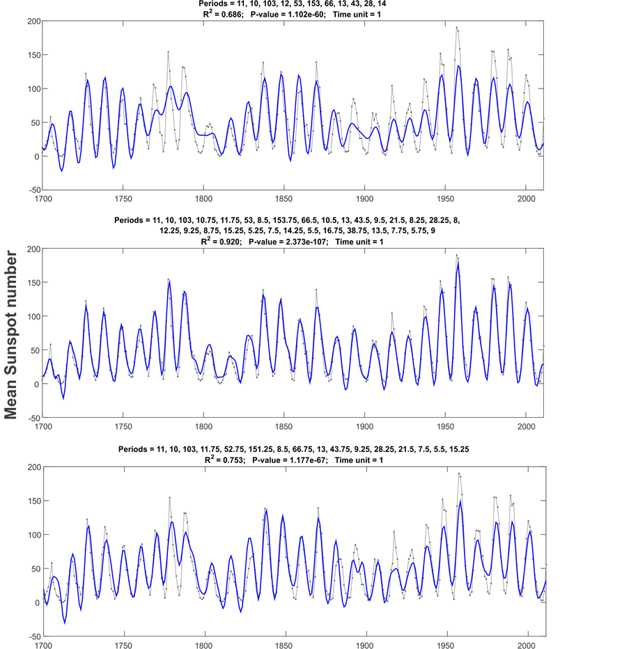
Figure 2. Yearly sunspot numbers from 1700 - 2011 and the periodicities found with Periods using three different options. Original series: black line with filled circles; fitted model: blue line. Upper panel shows the result of the default search (step = 1). In the middle panel, the search for periods was on a quarterly basis (step = 0.25). In the bottom panel, two upper and two lower quarterly optimum period neighbors were discarded with neig = 2.
To improve the fitted model and also to illustrate the flexibility of the Periods function, the sunspot series was reanalyzed using step = 0.25 in order to evaluate fractional (quarterly) sunspot cycles, since some authors have reported periods in fractions of years. The middle panel of Figure 2 illustrates this analysis, where the number of significant harmonics grow to 30 and the  (0.917) show an increase of 23%.
Periods with small differences between them may be regarded as closely related, for instance 5.25, 5.5 and 5.75. In some cases it may not be desirable to report cycles with such small differences. The neig argument can be used to remove neighboring values above and below a previously identified period preventing these values from being tested in subsequent steps of the cyclic descent. To illustrate this, the previous analysis was repeated adding neig = 2. The result is shown in the bottom panel of Figure 2. The Periods function now identifies only 16 significant harmonics at the expense of a lower  (0.753). This model is, nevertheless, simpler than the preceding and the fit is acceptable. The periods, amplitudes, phases and lags are in Table 2.
It must to be noted that the removal of neighboring periods is solely a user decision, and it is therefore subjective. It is up to the user to decide whether or not it makes sense to obtain all the possible periods in a given analysis or to limit the search to non-contiguous cycles. In any case, it is recommended to carry out some testing and compare the results before deciding on this matter. Other options that can be explored by the user are the inclusion or exclusion of periods depending on previous knowledge on the data (arguments: include, exclude). Again, this is only a user decision.
Also, it should be noticed that there is a slight difference in the arrangement and values of the harmonics and the R2 value found in the Cyclic Descent process and the fitted Final Model showed by the method. The reason for this is, once the Cyclic Descent process found a certain number of harmonics, these are used as seed values for fitting a model for the observed data, and there is a rearrangement of the found values, and usually there are slight changes in the values of harmonics, phases, etc., and in a slight increase in the R2 value of the fitted model.
There are other function arguments that the user can control to modify the behavior of Periods as explained in Section 0. Users are encouraged to explore the effect of changing the default values of these arguments in the
Table 2. Summary results from yearly sunspot series (1700 - 2011) analyzed with Periods(sunspots, year, step = 0.25, neig = 2). Harmonics are ordered according to their amplitudes and the first column corresponds to the order in which periods were found in the cyclic descent.
function output.
Comparing the 14 periods found by [14] with our results from the third analysis, we found nine matching periods. Seven have differences less than 0.2 years and two differ between 1.7 to 2.25 years. Figure 3 shows the periods reported by [14] and those found in this study arranged side by side and spaced vertically by decreasing amplitude (on a logarithmic scale). Similar periods are joined by lines, whose slopes are proportional to the magnitude of change of their corresponding amplitudes reflecting their relative importance in the time series.
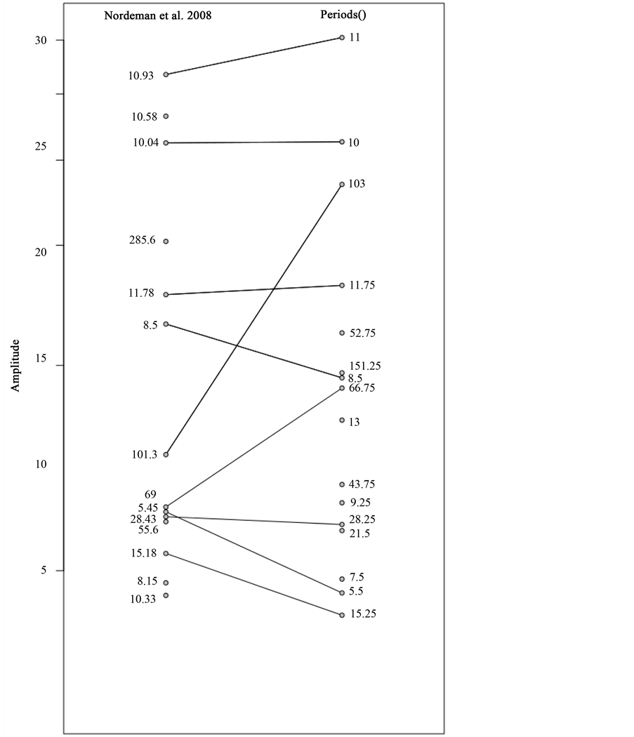
Figure 3. Comparison of the periods found in the sunspot time series by [14] (left) with those found in this study (right). Vertical arrangement of the periods is given by their corresponding decreasing amplitude (in logarithmic scale). See text for an explanation.
4.3. Multivariate ENSO Index
Another good example to test the Periods function with real data, is the MEI (Multivariate El Niño Southern Oscillation Index) time series, which is the first principal component of six variables3. This is a monthly series constructed to monitor El Niño/La Niña activity and intensity in the tropical Pacific Ocean from 1950 to date [15] [16] . There is a extended version for this index which goes back to 1871 [17] . For the purpose of this paper we used the regular index for the period 1950-2014. Several authors indicate that El Niño occurs on a 2 - 10 year time-scale [18] , being 3 - 6 the more common period reported [19] [20] . During the last decade, it has been recognized that the frequency and extent of this event is changing ( [21] ). Below we present three different analyses with Periods and compare our results with literature.
Again, a first analysis was carried out using the code.
>> [Final_model, Cyclic_Descent] = Periods (MEI, t)
The upper panel in Figure 4 shows the corresponding fitted model  with thirty-six significant
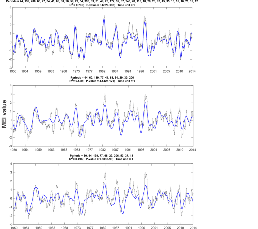
Figure 4. Multivariate ENSO Index (MEI) from 1950 - 2014 and the periodicities found with Periods using three different analysis. Original series: black line with filled circles; fitted model: blue line. Upper panel shows the result of the default search (step = 1). In the middle panel, the search for periods was carried out selecting the first ten highly significant periods (99.99%) using hn = 10 and alpha = 0.0001. In the lower panel, besides the discarding yearly neighbors (neig = 6) only the statistically significant periods at  are shown using alpha = 0.0001.
harmonics. Note that the 44-month period (3.6 years) is the first period found, and as in the Sunspot time series, it means that such period has the largest amplitude and therefore it is the most influential period in the time series. This period is followed by a 136 and a 60-month periods (11.6 and 5 years respectively), indicating the importance of those periods in the index.
It can be recognized that there are many periods with values close to each other. Therefore, if the user want to better discern between found periods, taking, for example, only the first ten highly significant periods, the MEI series can be reanalyzed using hn = 10 and alpha = 0.0001 in order to choose only the first ten periods significant at 99.99% . The middle panel of Figure 4 illustrates the results for this analysis, where the number of significant harmonics was reduced to 10, and also the
  (0.559) showed a decrease of 23.6%. This model is much simpler than the preceding and the fit might be considered as acceptable. However, in the latter analysis can be noted that there are some really close values than are somehow difficult to explain (e.g. 29 and 30-month periods). If the user wants to determine only the periods which are no adjacent to each other at least 12 months between them, and also choose only those which are significant at the same latter significance level, the series can be again reanalyzed using neig = 6 and alpha = 0.0001. The first option will ignore 6 months back and forth a found period, meanwhile the second option will retain only the periods significant at 99.99%. The lower panel of 4 shows the fit, periods and
  for this analysis. In such case, Periods function found 11 significant harmonics, and again with an acceptable
  (0.496). In this case, once a significant harmonic is found, the program ignores any other harmonic in a window of 12 months, and starts searching again for more significant harmonics The periods, amplitudes, phases and lags are in Table 3.
Most of cycles found by this method are already reported in literature. For example, the first period, the 60-month-cycle, has been already reported for MEI [22] , as a highly statistically significant period (>99%). Also, [23] reported that ENSO occurrence changed from high to low frequency (averaging 20 to 60 months) from 1960’s to 1990’s, showing periods from 2 - 4 years from 1962 to 1975 and 4 - 6 years from 1980 to 1993. It is also acknowledged that the MEI series shares the Pacific Decadal Oscillation signal [24] [25] , which lasts 20 - 30 years, and as in the latter case both periods are found in our analysis. However, there are 4 periods not well described in literature: 11.6, 14.3, 17.2 and 21-year. The first and latter could be related to solar sunspots cycles, however, the 14.3 and 17.2 years periods could just be a periodicity of the series that require more research. Also, unlike most of the results shown, this method provided the amplitud, phase and lag of every period found, which can be really useful in a detailed and more depth study.
It is worth noting the effect of removing neighboring periods. It makes the process of identifying close periods much clearer, reducing the number of found periods to a minimum. However, it is recommended to use the highest number of periods possible if the objective is forecasting beyond the time series. As stated in previous section, it is merely a user’s decision whether or not obtaining all the possible periods in a given
Table 3. Summary results from MEI series (1950-2014) analyzed with Periods (MEI, neig = 6, alpha = 0.0001). Harmonics are ordered according to their amplitudes and the first column corresponds to the order in which periods were found in the cyclic descent.
analysis or to limit the search to non-contiguous cycles and it is highly recommended to test and compare the results before deciding on this matter.
We are not implying that our results on the sunspot number cycles and multivariate ENSO index are more accurate than those from previous studies, however, we believe that the proposed function can be a useful exploratory tool for users who are not particularly trained in time series analysis.
The decomposition of a time series into several signals as proposed here is not unique. Several methods for this purpose have been proposed, for example the method of frames, matching pursuit and best orthogonal basis [4] among others. However, the Periods function is quite simple and easy to understand, which in turn allows its immediate use by the average or occasional user, who wishes finding periodicities in his or her data and to relate them to environmental or other nature indexes.
5. Remarks
The main advantages of the Periods function are the following: full description of the harmonics by their three parameters, amplitude, period and phase, including the lag phase that permits an easy graphical interpretation useful to compare lags between several responses of the same phenomenon. The output periodicities of the cyclic descent method can be interpreted or related to other known periodic events, because they are found sequentially to give their order of importance in explaining the residuals. This order and the lag can be relevant in such interpretations. For forecasting purposes, the final fitted model will be more useful because of its best statistical significance. The fitted parameters can be slightly different to those of the cyclic descent, especially the amplitudes, which indicates the relative importance of the harmonics in the fitted model (Table 2). Due to its simplicity and flexibility, the Periods function can be an important exploratory tool for time series analysis.
The Periods function can be requested for free use to the corresponding author. Furthermore, there is a R version for the users with no access to MATLAB. Feel free to use both versions and distribute them.
Acknowledgements
We want to thank D. Lluch-Belda (+) for the support and comments for this paper. EGR and VMGM are grant holders of the Sistema Nacional de Investigadores (CONACYT). VMGM and HV were supported by a fellowship from COFAA-IPN. EGR and ARR want to thank CICESE ULP for the support provided.
Cite this paper
Eduardo González-Rodríguez,Héctor Villalobos,Víctor Manuel Gómez-Muñoz,Alejandro Ramos-Rodríguez, (2015) Computational Method for Extracting and Modeling Periodicities in Time Series. Open Journal of Statistics,05,604-617. doi: 10.4236/ojs.2015.56062
References
- 1. Bloomfield Fourier, P. (1976) Analysis of Time Series: An Introduction. 1st Editon, John Wiley and Sons, Hoboken.
- 2. Lluch-Belda, D., Lauks, M., Lluch-Cota, D.B. and Lluch-Cota, S.E. (2001) Long-Term Trends of Interannual Variability in the California Current System. CalCOFI Reports, 42, 129-144.
- 3. Mallat, S.G. and Zhang, Z. (1993) Matching Pursuits with Time-Frequency Dictionaries. IEEE Transactions on Signal Processing, 41, 3397-3415.
http://dx.doi.org/10.1109/78.258082 - 4. Chen, S.S., Donoho, D.L. and Saunders, M.A. (1998) Atomic Decomposition by Basis Pursuit. SIAM Journal on Scientific Computing, 20, 33-61.
http://dx.doi.org/10.1137/S1064827596304010 - 5. Bliss, C.I. (1958) Periodic Regression in Biology and Climatology. New Haven, Connecticut Agricultural Experiment Station Bulletin, 612, 55 p.
- 6. Bloomfield Fourier, P. (2000) Analysis of Time Series: An Introduction. 2nd Edition, John Wiley and Sons, Hoboken.
- 7. Kammler, D.W. (2008) A First Course in Fourier Analysis. Cambridge University Press, Cambridge.
- 8. Draper, N.R. and Smith, H. (1998) Applied Regression Analysis. John Wiley and Sons, Hoboken.
- 9. Hathaway, D.H., Wilson, R.M. and Reichmann, E.J. (2002) Group Sunspot Numbers: Sunspot Cycle Characteristics. Solar Physics, 211, 357-370.
http://dx.doi.org/10.1023/A:1022425402664 - 10. Berry, P.A.M. (1987) Periodicities in the Sunspot Cycle. Vistas in Astronomy, 30, 97-108.
http://dx.doi.org/10.1016/0083-6656(87)90011-0 - 11. Rozelot, J.P. (1993) On the Periodicities in the Solar Cycle. Advances in Space Research, 13, 439-442.
http://dx.doi.org/10.1016/0273-1177(93)90516-E - 12. Lamb, H.H. (1972) Climate:Present, Past and Future. Methuen and Co. Ltd, London.
- 13. Herman, J.R. and Goldberg, R.A. (1985) Sun, Weather and Climate. Dover Publications Inc., New York.
- 14. Nordemann, D.J.R., Rigozo, N.R., de-Souza-Echer, M.P. and Echer, E. (2008) Principal Components and Iterative Regression Analysis of Geophysical Series: Application to Sunspot Number (1750-2004). Comput Geosciences, 34, 1443-1453.
http://dx.doi.org/10.1016/j.cageo.2007.09.022 - 15. Wolter, K. and Timlin, M.S. (1993) Monitoring ENSO in COADS with a Seasonally Adjusted Principal Component Index. Proceedings of the 17th Climate Diagnostics Workshop, Norman, January 1993, 52-57.
- 16. Wolter, K. and Timlin, M.S. (1998) Measuring the Strength of ENSO Events: How Does 1997/98 Rank? Weather, 53, 315-324.
http://dx.doi.org/10.1002/j.1477-8696.1998.tb06408.x - 17. Wolter, K. and Timlin, M.S. (2011) El Niño/Southern Oscillation Behaviour Since 1871 as Diagnosed in an Extended Multivariate ENSO Index (MEI.ext) International Journal of Climatology, 31, 1074-1087.
http://dx.doi.org/10.1002/joc.2336 - 18. Trenberth, K.E. and Shea, D.J. (1987) On the Evolution of Southern Oscillation. Monthly Weather Review, 115, 3078-3096. http://dx.doi.org/10.1175/1520-0493(1987)115<3078:OTEOTS>2.0.CO;2
- 19. Trenberth, K.E. (1997) The Definition of El Niño. Bulletin of the American Meteorological Society, 78, 2771-2077.
http://dx.doi.org/10.1175/1520-0477(1997)078<2771:TDOENO>2.0.CO;2 - 20. Philander, S.G. and Fedorov, A. (2003) Is El Niño Sporadic or Cyclic? Annual Review of Earth and Planetary Sciences, 31, 579-594.
http://dx.doi.org/10.1146/annurev.earth.31.100901.141255 - 21. Cai, W., Borlace, S., Lengaigne, M., van Rensch, P., Collins, M., Vecchi, G., Timmermann, A., Santoso, A., McPhaden, M.J., Wu, L., England, M.H., Wang, G., Guilyardi, E. and Jin, F. (2000) Increasing Frequency of Extreme El Niño Events Due to Greenhouse Warming. Nature Climate Change, 4, 111-116.
http://dx.doi.org/10.1038/nclimate2100 - 22. Mazzarella, A., Giuliacci, A. and Liritzis, I. (2010) On the 60-Month Cycle of Multivariate ENSO Index. Theoretical and Applied Climatology, 100, 23-27.
http://dx.doi.org/10.1007/s00704-009-0159-0 - 23. An, S. and Wang, B. (2000) Interdecadal Change of the Structure of the ENSO Mode and Its Impact on the ENSO Frequency. Journal of Climate, 13, 2044-2055.
- 24. Mantua, N.J., Hare, S.R., Zhang, Y., Wallace, J.M. and Francis, R.C. (1997) A Pacific Interdecadal Climate Oscillation with Impacts on Salmon Production. Bulletin of the American Meteorological Society, 78, 1069-1079.
http://dx.doi.org/10.1175/1520-0477(1997)078<1069:APICOW>2.0.CO;2 - 25. Alexander, M.A., Blade, I., Newman, M., Lanzante, J.R., Lau, N. and Scott, J.D. (2002) The Atmospheric Bridge: The Influence of ENSO Teleconnections on Air—Sea Interaction over the Global Oceans. Journal of Climate, 15, 2205-2231.
http://dx.doi.org/10.1175/1520-0442(2002)015<2205:TABTIO>2.0.CO;2
NOTES

1The statistical toolbox is required. The varargin parameters must be declared previously and the names must be exactly as they are defined.

