American Journal of Computational Mathematics
Vol.3 No.1(2013), Article ID:29524,6 pages DOI:10.4236/ajcm.2013.31013
Existence the Solutions of Some Fifth-Order Kdv Equation by Laplace Decomposition Method
1Department of Mathematics, Mahatma Basweshwar Mahavidyalaya, Latur, India
2Department of Mathematics, Maharashtra Udaygiri Mahavidyalaya, Udgir, India
Email: sujitmaths@gmail.com
Received October 14, 2012; revised November 30, 2012; accepted December 10, 2012
Keywords: Laplace Decomposition Method; Nonlinear Partial Differential Equations; Fifth-Order Kdv Equation; The Kawahara Equation
ABSTRACT
In this paper, we develop a method to calculate numerical and approximate solution of some fifth-order Korteweg-de Vries equations with initial condition with the help of Laplace Decomposition Method (LDM). The technique is based on the application of Laplace transform to some fifth-order Kdv equations. The nonlinear term can easily be handled with the help of Adomian polynomials. We illustrate this technique with the help of four examples and results of the present technique have closed agreement with approximate solutions obtained with the help of (LDM).
1. Introduction
The theory of nonlinear dispersive wave motion has recently undergone much study. We do not attempt to characterize the general form of nonlinear dispersive wave equations [1]. Rather, we solve a specific equation in the following nonlinear Equation (1) by using the Laplace decomposition method (LDM) [2]. Nonlinear phenomena play a crucial role in applied mathematics and physics. Furthermore, when an original nonlinear equation is directly calculated, the solution will preserve the actual physical characters of solutions [3]. There are many standard methods in literature to solve the fifthorder Korteweg-de Vries (FKdV) equations. Explicit solutions to the nonlinear equations are of fundamental importance. Various methods for obtaining explicit solutions to nonlinear evolution equations have been proposed. Among them are Hirota’s dependent variable transformation, the inverse scattering transform, and the Bcklund transformation. All these methods are described in [1,4] and the references therein. A feature common to all these methods is that they are using the transformations to reduce the equation into more simple equation then solve it. Unlike classical techniques, the nonlinear equations are solved easily and elegantly without transforming the equation by using the LDM. The LDM is providing an efficient explicit and numerical solutions with high accuracy, minimal calculation, avoidance of physically unrealistic assumptions.
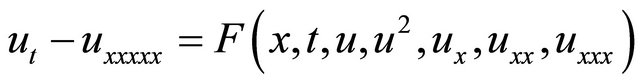
We now describe how the Laplace decomposition method can be used to construct the solution to the initial-value problem for the FKdV equation [1,4-6],
 (1)
(1)
which occurs, for example, in the theory of magnetoacoustic waves in plasmas [6] and in the theory of shallow water waves with surface tension [7]. The FKdV equation has been investigated extensively over last decade. It has been shown that the travelling-wave solutions of this equation do not vanish at infinity [8,9].
In this paper, we generated an appropriate Adomian’s polynomials for the generalized a FKdV Equation (1). The solution of the equations, homogeneous or inhomogeneous, will be handle more easily, quickly, and elegantly by implementing the LDM rather than the traditional methods for the approximate and numerical solutions of which are to be obtained subject to the initial condition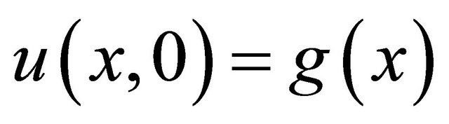 .
.
2. Laplace Decomposition Method
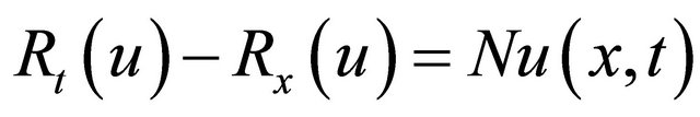
Let us consider the standard form of a FKdV Equation (1) in an operator form
 (2)
(2)
with initial condition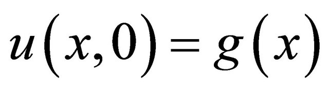 .
.
Where the notation ,
,  symbolize the linear differential operators and
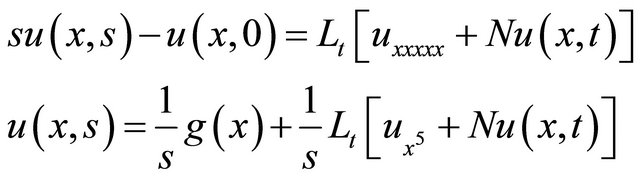
  represent the general nonlinear term. Taking the Laplace transform of Equation (2) with respect to t, we get
 (3)
(3)
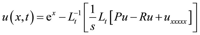
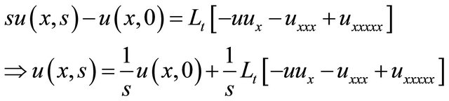
Taking inverse Laplace transform of Equation (3) with respect to “t”, we get,
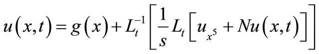 (4)
(4)
In Laplace decomposition method we represent solution in infinite series form.Therefore suppose that
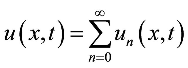 (5)
(5)
is the required solution of Equation (1). A nonlinear term contained in Equation (2), we can decompose it by using adomian polynomial. Its formula is given below
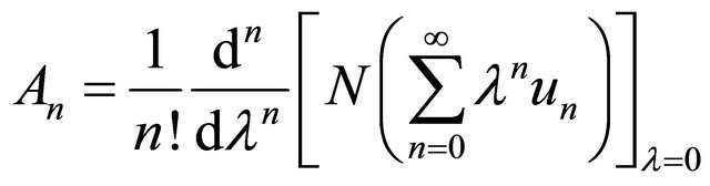 (6)
(6)
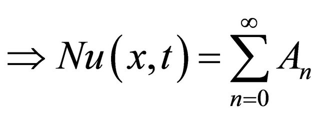 (7)
(7)
where  are Adomian polynomials of
 , n
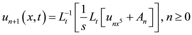
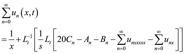
, n 0. Which are calculated by using Equation (6). From Equations (4), (5) and (7) we get
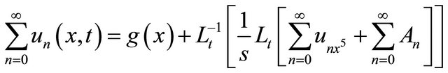 (8)
(8)
comparing both sides of Equation (6), we get a recursive relation
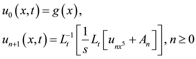 (9)
(9)
In the following section we have given the some examples with absolute errors , where
  is the particular exact solution and
  is the partial sums
 (10)
(10)
It is clear from Equations (9) and (10), we get
 (11)
(11)
Moreover, the decomposition series (1) solutions are generally converge very rapidly in real physical problems [3,10]. The convergence of the decomposition series have investigated by several authors. The theoretical treatment of convergence of the decomposition method has been considered in [11-13]. They obtained some results about the speed of convergence of this method providing us to solve linear and nonlinear functional equations Recently, Wazwaz [14] proposed that the construction of the zeroth component of the decomposition series can be define in a slightly different way. In [14], he assumed that if the zeroth component is , the function g is possible to divide into two parts such as
  and
and , then one can formulate the recursive algorithm
 . The same idea we can use in LDM . The Equation (9) general term in a form of the modified recursive scheme as follows:
 (12)
(12)
 (13)
(13)
 (14)
(14)
This type of modification is giving more flexibility to the modified Laplace decomposition method (MLDM) in order to solve complicate nonlinear differential equations. In many case the modified scheme avoids the unnecessary computations, especially in calculation of the Adomian polynomials. Furthermore, sometimes we do not need to evaluate the so-called Adomian polynomials or if we need to evaluate these polynomials the computation will be reduced very considerably by using the modified recursive scheme. For more details of this MLDM, one can see Ref. [14,15]. Illustration purpose we will consider both homogeneous and inhomogeneous FKdV equations in the following section. We will show that how the MLDM is computationally efficient.
3. Applications and Result
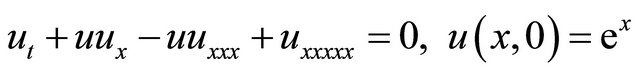
Example 1: Consider the following FKdV Equation (1) is given with the initial condition
 (15)
(15)
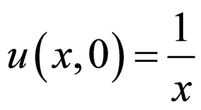 (16)
(16)
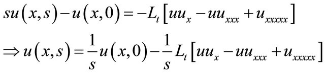
Taking the Laplace transform of Equation (15) with respect to “t”, we get
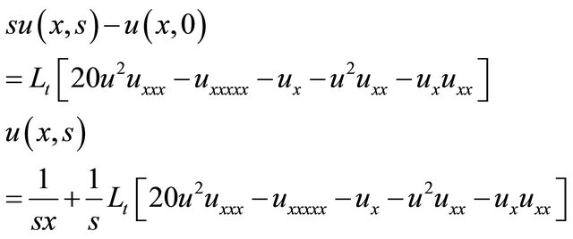 (17)
(17)
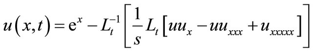
Taking the inverse Laplace transform of Equation (17) with respect to “t”, we get
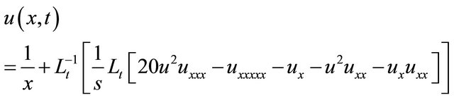 (18)
(18)
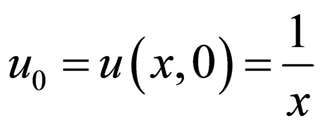
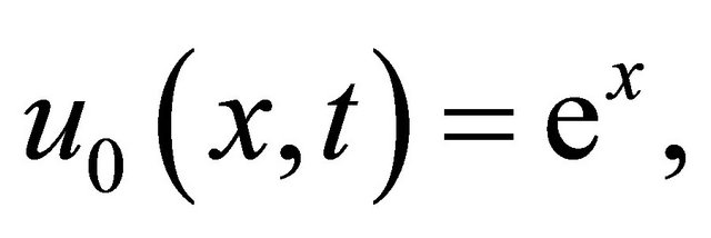
Since initial value is known and decompose the unknown function  a sum of components defined by the decomposition series (5) with
  identified as
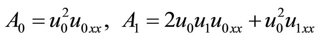
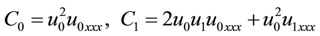
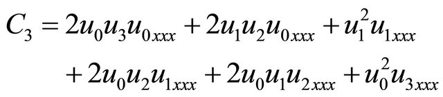
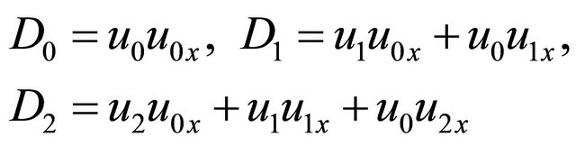
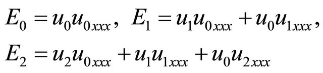
 . An important part of the method is to express the Adomian’s polynomials; thus
 ,
,  , and
, and  are the appropriate Adomian’s polynomials which are generated by using general formula (6) for the above example as in the form of
 (19)
(19)
 (20)
(20)
 (21)
(21)
 (22)
(22)
 (23)
(23)
 (24)
(24)
 (25)
(25)
 (26)
(26)
 (27)
(27)
and so on for other polynomials can be obtained in a similar manner.
The Equation (18) we can write in the following form also
 (28)
(28)
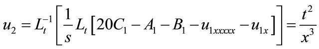
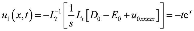
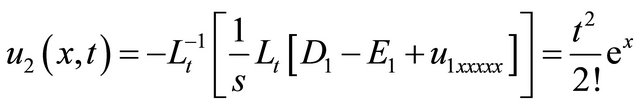
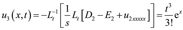
Comparing the both sides of Equation (28), we get the term-by-term components,
 (29)
(29)
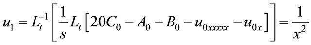 (30)
(30)
 (31)
(31)
 (32)
(32)
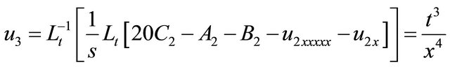
and so on, in this manner the rest of components of the decomposition series were obtained. Substituting (29)- (32) into (5) gives the solution  in a series from and in a closed form by
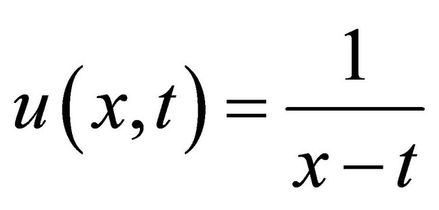 .
.
Example 2: Consider an equation with initial condition is given by
 (33)
(33)
Taking the Laplace transform of Equation (33) with respect to t, we get
 (34)
(34)
Taking inverse Laplace transform of Equation (34) with respect to t, we get
 (35)
(35)
The nonlinear terms contained in Equation (33), we con decompose it by using Adomian’s polynomials. Let 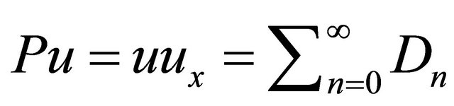 and
and 
Thus, the Equation (35) becomes,
 (36)
(36)
The Adomian’s polynomials  and
and  are calculated by using the formula (6) for the second example as in the form of
 (37)
(37)
 (38)
(38)
and so on for other polynomials can be calculated in similar manner. By using Equation (9) with Adomian polynomials (37) and (38) to determine the other individual terms of the decomposition series, we find
 (39)
(39)
 (40)
(40)
 (41)
(41)
 (42)
(42)
and so on, in this manner the rest components of the decomposition series were obtained. Substituting the value of (39)-(42) into the Equation (5) gives the solution  in a series form and in a close form by
 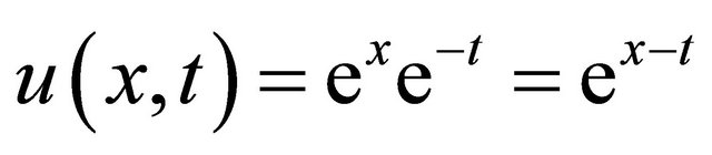 . Which can be verified through substitution.
Example 3: We consider the Kawahara equation [5]
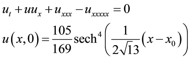 (43)
(43)
Taking Laplace transform on both sides of Equation (45) with respect to t, we get
 (44)
(44)
Taking inverse Laplace transform of Equation (44) with respect to t, we get
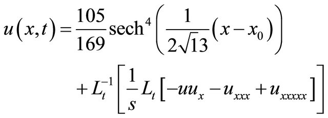 (45)
(45)
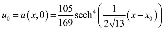
Since the nonlinear term contain in Equation (43), we can decompose it by using the Adomian polynomial (6). Suppose that . Decompose the unknown function
  a sum of components defined by the decomposition series (5) with u0 identified with
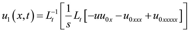
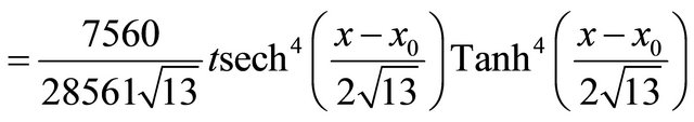
 . The other components of the decomposition series (5) can be compute by using recursive relation (9) with the Adomian polynomials (37), we get the following components
 (46)
(46)
 (47)
(47)
 (48)
(48)
 (49)
(49)
 (50)
(50)
 (51)
(51)
 (52)
(52)
 (53)
(53)
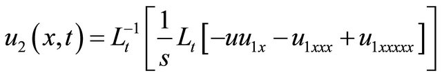
and so on, in this manner the rest of components of the decomposition series were obtain. Substituting (46), (48), (52) into (5) gives the solution  in a series form and in a close form by
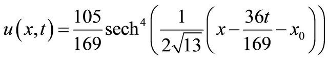 (54)
(54)
This result can be verify through substitution.
Example 4: As an example of the application of the self-canceling phenomena [14,16,17], let us seek the explicit solution of the nonhomogeneous FKdV equation with initial condition:
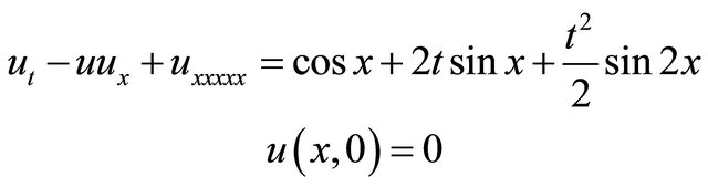 (55)
(55)
To obtain the decomposition solution subject to initial condition given, we first use (52) in an operator form in the same manner as form (2) and then we used (9) to determine the individual terms of the decomposition series, we get immediately
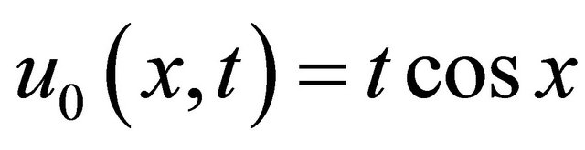 (56)
(56)
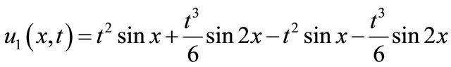 (57)
(57)
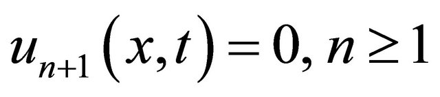 (58)
(58)
It is obvious that the noise terms appear between the components of u1, and these are all canceled.As seen Equation (57), the closed form of the solution can be find very easily by proper selection of g1 and g2. In the case of right choice of these functions, the modified technique accelerate the convergence of the decomposition series solution by computing just u0 and u1 terms of the series. The term u0 provides the exact solution as  and this can be justifies through substitution.This has been justified by [14,15].
4. Experimental Results
In order to verify numerically whether the proposed methodology lead to higher accuracy, we can evaluate the numerical solutions using the n-term approximation (10). Tables 1-3 show the difference of the analytical solution and numerical solution of the absolute errors. It is to be note that five terms only were used in evaluating the approximate solutions. We achieved a very good approximation with the actual solution of the equations by using five terms only of the decomposition derived above. It is evident that the overall errors can be made smaller by adding new terms of the decomposition series (5).
Numerical approximations show a high degree of accuracy and in most cases , the n-term approximation is accurate for quite low values of n.
Table 1. The numerical results for  in comparison with the analytical solution
  for the rational solutions of the Equation (15).
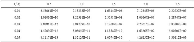
Table 2. The numerical results for  in comparison with the analytical solution
  for the rational solutions of the Equation (33).
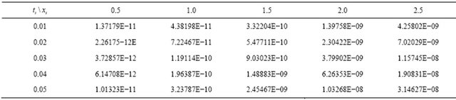
Table 3. The numerical results for  in comparison with the analytical solution
 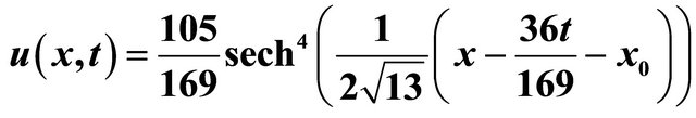 when
when , for the travelling-wave solution of the Equation (43).
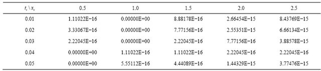
The solutions are very rapidly convergent by utilizing the LDM.The numerical results we obtained justify the advantage of this methodology, even in the few terms approximation is accurate. Furthermore, as the decomposition method does not require discretization of the variables, i.e. time and space, it is not affected by computation round off errors and one is not faced with necessity of large computer memory and time.
5. Conclusions
In conclusion, the Laplace decomposition method was used for finding the exact solution and approximate solution of the FKdV (1). The method can be also easy to be extended to other nonlinear evaluation equations, with the aid of Mathematica (or Matlab, Maple, Reduce, etc.)the course of solving nonlinear evaluation equations can be carried out in computer. Four coupled nonlinear FKdV equations with initial conditions are discussed as Laplace demonstrations method. It may be consulated that the Laplace decomposition method is very powerful and efficient technique in finding exact solutions for wide classes of problems. It is also worth nothing to point out that the advantage of the Laplace decomposition method is the fast convergence of the solutions. A fast convergence of the solution may be achieved by observing the self-canceling noise terms and a proper selection of g1 and g2, the demonstration of this case is shown in Example 4.
Finally, we point out that, for given equations with initial values , the corresponding analytical and numerical solutions are obtained according to the recurrence relations (9) using Mathematica [18].
REFERENCES
- P. G. Drazin and R. S. Johnson, “Solutions: An Introduction,” Cambridge University Press, Cambridge, 1989. doi:10.1017/CBO9781139172059
- M. Khan, “Application of Laplace Decomposition Method to Solve Nonlinear Coupled Partial Differential Equations,” World Applied Sciences Journal, Vol. 9, 2010, pp. 13-19.
- G. Adomian, “A Review of the Decomposition Method in Applied Mathematics,” Journal of Mathematical Analysis and Applications, Vol. 135, No. 2, 1988, pp. 501-544.
- X. Q. Liu and C. L. Bai, “Exact Solutions of Some FifthOrder Nonlinear Equations,” Applied Mathematics—A Journal of Chinese Universities, Vol. 15, No. 1, 2000, pp. 28-32.
- E. J. Parkes and B. R. Duffy, “An Automated Tanh-Function Method for Finding Solitary Wave Solutions to NonLinear Evolution Equations,” Computer Physics Communications, Vol. 98, No. 3, 1996, pp. 288-300. doi:10.1016/0010-4655(96)00104-X
- T. R. Akylas and T.-S. Yang, “On Short-Scale Oscillatory Tails of Long-Wave Disturbances,” Studies in Applied Mathematics, Vol. 94, 1995, pp. 1-20.
- J. K. Hunter and J. Scheurle, “Existence of Perturbed Solitary Wave Solutions to a Model Equation for Water Waves,” Physica D: Nonlinear Phenomena, Vol. 32, No. 2, 1988, pp. 253-268. doi:10.1016/0167-2789(88)90054-1
- J. P. Body, “Weak Non-Local Solitons for CapillaryGravity Waves: Fifth-Order Korteweg-de Vries Equation,” Physica D, Vol. 48, 1991, pp. 129-146.
- J. T. Beale, “Exact Solitary Waves with Capillary Ripples at Infinity,” Communications Pure Applied Mathematics, Vol. 44, 1991, pp. 211-247.
- G. Adomian, “Solving Frontier Problems of Physics: The Decomposition Method,” Kluwer Academic Publishers, Boston, 1994.
- Y. Cherruault, “Convergence of Adomian’s Method,” Kybernetics, Vol. 18, 1989, pp. 31-38.
- A. Repaci, “Nonlinear Dynamical Systems: On the Accuracy of Adomian’s Decomposition Method,” Applied Mathematics Letters, Vol. 3, No. 4, 1990, pp. 35-39.
- Y. Cherruault and G. Adomian, “Decomposition Methods: A New Proof of Convergence,” Mathematical and Computer Modelling, Vol. 18, No. 12, 1993, pp. 103-106. doi:10.1016/0895-7177(93)90233-O
- A. M. Wazwaz, “A Reliable Modification of Adomian Decomposition Method,” Applied Mathematics and Computation, Vol. 102, No. 1, 1999, pp. 77-86. doi:10.1016/S0096-3003(98)10024-3
- M. Hussain, “Modified Laplace Decomposition Method,” Applied Mathematical Science, Vol. 4, No. 38, 2010, pp. 1769-1783.
- G. Adomian and R. Rach, “Noise Terms in Decomposition Solution Series,” Applied Mathematics and Computation, Vol. 24, No. 11, 1992, pp. 61-64.
- A. M. Wazwaz, “Necessary Conditions for the Appearance of Noise Terms in Decomposition Solution Series,” Applied Mathematics and Computation, Vol. 81, No. 2-3, 1997, pp. 265-274.
- S. Wolfram, “Mathematica for Windows,” Wolfram Research Inc., Champaign, 1993.