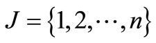
American Journal of Operations Research
Vol.3 No.6(2013), Article ID:40056,8 pages DOI:10.4236/ajor.2013.36055
Linear Plus Linear Fractional Capacitated Transportation Problem with Restricted Flow
1Department of Mathematics, Ramjas College, University of Delhi, Delhi, India
2Department of Mathematics, Hans Raj College, University of Delhi, Delhi, India
Email: gupta_kavita31@yahoo.com, srarora @yahoo.com
Copyright © 2013 Kavita Gupta, Shri Ram Arora. This is an open access article distributed under the Creative Commons Attribution License, which permits unrestricted use, distribution, and reproduction in any medium, provided the original work is properly cited.
Received October 6, 2013; revised November 6, 2013; accepted November 13, 2013
Keywords: Transportation Problem; Linear Plus Linear Fractional; Restricted Flow; Corner Feasible Solution
Abstract
In this paper, a transportation problem with an objective function as the sum of a linear and fractional function is considered. The linear function represents the total transportation cost incurred when the goods are shipped from various sources to the destinations and the fractional function gives the ratio of sales tax to the total public expenditure. Our objective is to determine the transportation schedule which minimizes the sum of total transportation cost and ratio of total sales tax paid to the total public expenditure. Sometimes, situations arise where either reserve stocks have to be kept at the supply points, for emergencies or there may be extra demand in the markets. In such situations, the total flow needs to be controlled or enhanced. In this paper, a special class of transportation problems is studied where in the total transportation flow is restricted to a known specified level. A related transportation problem is formulated and it is shown that to each basic feasible solution which is called corner feasible solution to related transportation problem, there is a corresponding feasible solution to this restricted flow problem. The optimal solution to restricted flow problem may be obtained from the optimal solution to related transportation problem. An algorithm is presented to solve a capacitated linear plus linear fractional transportation problem with restricted flow. The algorithm is supported by a real life example of a manufacturing company.
1. Introduction
Transportation problems with fractional objective function are widely used as performance measures in many real life situations such as the analysis of financial aspects of transportation enterprises and undertaking, and transportation management situations, where an individual, or a group of people is confronted with the hurdle of maintaining good ratios between some important and crucial parameters concerned with the transportation of commodities from certain sources to various destinations. Fractional objective function includes optimization of ratio of total actual transportation cost to total standard transportation cost, total return to total investment, ratio of risk assets to capital, total tax to total public expenditure on commodity etc. Gupta, Khanna and Puri [1] discussed a paradox in linear fractional transportation problem with mixed constraints and established a sufficient condition for the existence of a paradox. Jain and Saksena [2] studied time minimizing transportation problem with fractional bottleneck objective function which is solved by a lexicographic primal code. Xie, Jia and Jia [3] developed a technique for duration and cost optimization for transportation problem. In addition to this fractional objective function, if one more linear function is added, then it makes the problem more realistic. This type of objective function is called linear plus linear fractional objective function. Khuranaand Arora [4] studied linear plus linear fractional transportation problem for restricted and enhanced flow.
Capacitated transportation problem finds its application in a variety of real world problems such as telecommunication networks, production-distribution systems, rail and urban road systems where there is scarcity of resources such as vehicles, docks, equipment capacity etc. Many researchers like Gupta and Arora [5], Misra and Das [6] have contributed to this field. Jain and Arya [7] studied the inverse version of capacitated transportation problem.
Many researchers like Arora and Gupta [8], Khurana, Thirwani and Arora [9] have studied restricted flow problems. Sometimes, situations arise when reserve stocks are to be kept at sources for emergencies. This gives rise to restricted flow problem where the total flow is restricted to a known specified level. This motivated us to develop an algorithm to solve a linear plus linear fractional capacitated transportation problem with restricted flow.
2. Problem Formulation
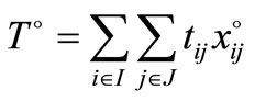
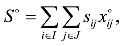
(P1): 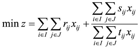
subject to
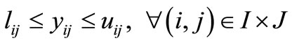
 (1)
(1)
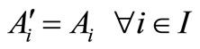
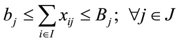 (2)
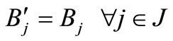
(2)
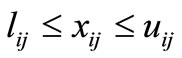 and integers
  (3)
(3)
 (4)
(4)
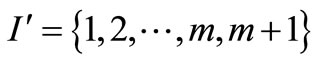
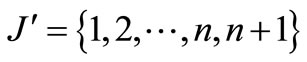
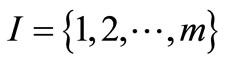 is the index set of m origins.
 is the index set of n destinations.
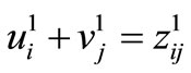
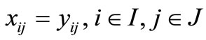
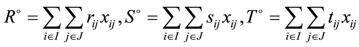
xij = number of units transported from origin i to destination j.
rij = per unit transportation cost when shipment is sent from ith origin to the jth destination.
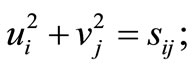
sij = the sales tax per unit of goods transported from ith origin to the jth destination.
tij = the total public expenditure per unit of goods transported from ith origin to the jth destination.
lij and uij are the bounds on number of units to be transported from ith origin to jth destination.
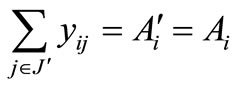
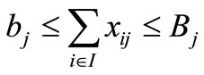
ai and Ai are the bounds on the availability at the ith origin, i  I bj and Bj are the bounds on the demand at the jth destination, j
  J It is assumed that
  for every feasible solution X satisfying (1), (2), (3) and (4) and all upper bounds uij;
  are finite.
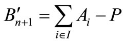
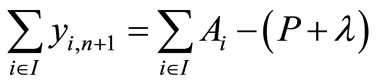
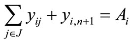
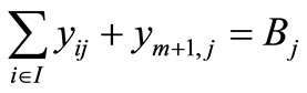
Sometimes, situations arise when one wishes to keep reserve stocks at the origins for emergencies, there by restricting the total transportation flow to a known specified level, say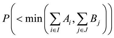 . This flow constraint in the problem (P1) implies that a total
 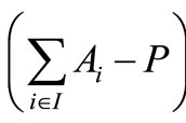 of the source reserves has to be kept at the various sources and a total
 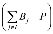 of destination slacks is to be retained at the various destinations. Therefore an extra destination to receive the source reserves and an extra source to fill up the destination slacks are introduced.
In order to solve the problem (P1) we convert it in to related problem (P2) given below.
(P2): 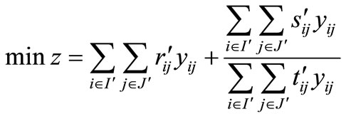
subject to


 ,
,
 ,
,  ,
, 
 ,
,
 ,
, 
 ,
,
 ,
, 
 ,
,
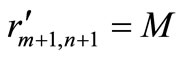
 ;
; 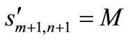
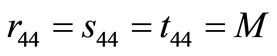
where M is a large positive number.
 ,
, 
3. Theoretical Development
Theorem1: A feasible solution 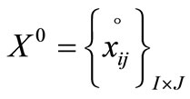 of problem (P1) with objective function value
  will be a local optimum basic feasible solution iff the following conditions holds.
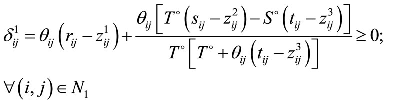
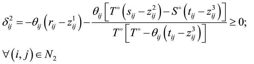
and if X0 is an optimal solution of (P2), then
 and
and 
where
 ,
, 
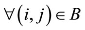
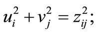
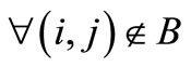
 B denotes the set of cells (i, j) which are basic and N1 and N2 denotes the set of non-basic cells (i, j) which are at their lower bounds and upper bounds respectively.
 are the dual variables such that
 ;
;
 ;
; ;
;
 ;
;
 ;
; .
.
Proof: Let  be a basic feasible solution of problem (P1) with equality constraints. Let z0 be the corresponding value of objective function. Then

Let some non-basic variable  undergoes change by an amount
  where
where  is given by
Then new value of the objective function  will be given by
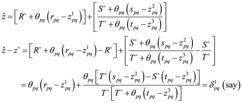
Similarly, when some non-basic variable  undergoes change by an amount
  then
then

Hence X0 will be local optimal solution iff  and
and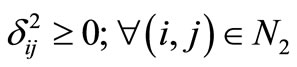 . If X0 is a global optimal solution of (P2), then it is an optimal solution and hence the result follows.
Definition: Corner feasible solution: A basic feasible solution  to(P2) is called a corner feasible solution (cfs) if
Theorem 2. A non-corner feasible solution of (P2) cannot provide a basic feasible solution to (P1).
Proof: Let  be a non-corner feasible solution to (P2). Then
Thus

Therefore,
Now, for ,
,
The above two relations implies that 
This implies that total quantity transported from all the sources in I to all the destinations in J is , a contradiction to the assumption that total flow is P and hence
  cannot provide a feasible solution to (P1).
Lemma1: There is a one-to-one correspondence between the feasible solution to (P1) and the corner feasible solution to (P2).
Proof: Let  be a feasible solution of (P1). So
 will satisfy (1) to (4).
Define  by the following transformation


It can be shown that  so defined is a cfs to (P2)
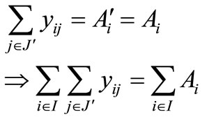
Relation (1) to (3) implies that


 Also for
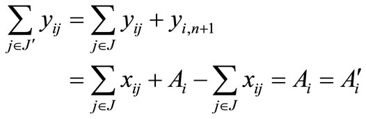
For 

Similarly, it can be shown that 
Therefore,  is a cfs to (P2).
Conversely, let  be a cfs to (P2). Define
 by the following transformation.
It implies that 
Now for , the source constraints in (P2) implies
 (since
 ).
).
Hence, 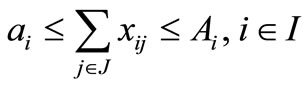
Similarly, for ,
, 
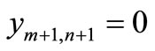
For i = m + 1,

 (because
 )
)
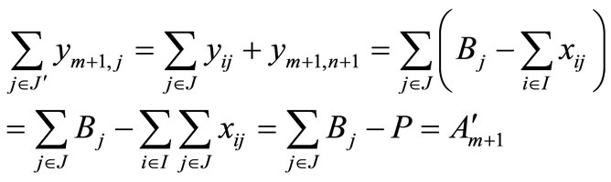
Now, for  the destination constraints in (P2) give
Therefore, 


Therefore  is a feasible solution to (P1)
Remark 1: If (P2) has a cfs, then since  and
and , it follows that non corner feasible solution cannot be an optimal solution of (P2).
Lemma 2: The value of the objective function of problem (P1) at a feasible solution  is equal to the value of the objective function of (P2) at its corresponding cfs
  and conversely.
Proof: The value of the objective function of problem
(P2) at a feasible solution  is
is
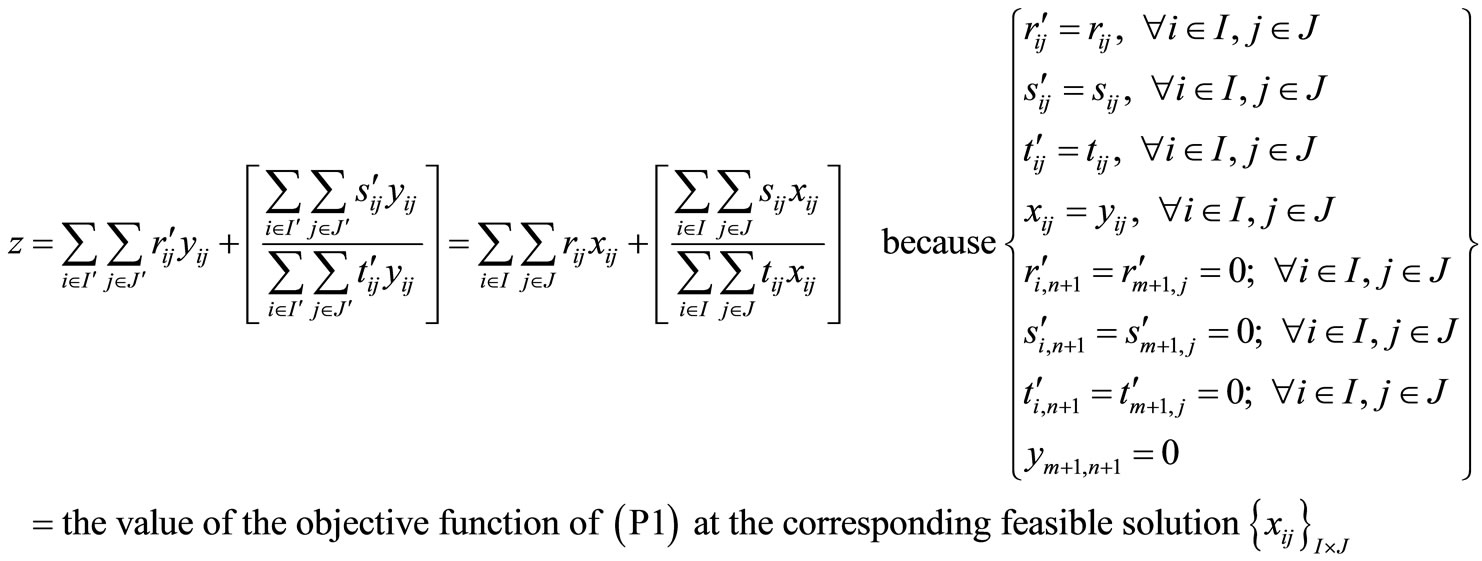
The converse can be proved in a similar way.
Lemma 3: There is a one-to-one correspondence between the optimal solution to (P1) and optimal solution to the corner feasible solution to (P2).
Proof: Let  be an optimal solution to (P1)yielding objective function value z0 and
  be the corresponding cfs to (P2).Then by Lemma 2, the value yielded by
 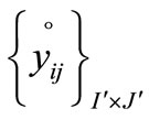 is z0. If possible, let
  be not an optimal solution to (P2) . Therefore, there exists a cfs
  say, to (P2) with the value z1 < z0 Let
  be the corresponding feasible solution to (P1).Then by Lemma 2,
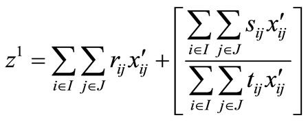
a contradiction to the assumption that  is an optimal solution of (P1).Similarly, an optimal corner feasible solution to (P2) will give an optimal solution to (P1).
Theorem 3: Optimizing (P2) is equivalent to optimizing (P1) provided (P1) has a feasible solution.
Proof: As (P1) has a feasible solution, by Lemma1, there exists a cfs to (P2). Thus by Remark 1, an optimal solution to (P2) will be a cfs. Hence, by Lemma 3, an optimal solution to (P1) can be obtained.
4. Algorithm
Step 1: Given a linear plus linear fractional capacitated transportation problem (P1), form a related transportation problem (P2). Find a basic feasible solution of problem (P2) with respect to variable cost only. Let B be its corresponding basis.
Step 2:
Calculate ,
,

such that
 ;
;

 = level at which a non-basic cell (i,j) enters the basis replacing some basic cell of B.
 are the dual variables which are determined by using the above equations and taking one of the ui’s or vj’s. as zero.
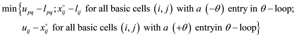
Step 3: Calculate  where
where
Step 4: Find  and
and 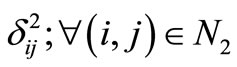 where
where

and
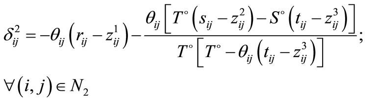
where N1 and N2 denotes the set of non-basic cells (i,j) which are at their lower bounds and upper bounds respectively.
If  and
and  then the current solution so obtained is the optimal solution to (P2) and subsequently to (P1). Then go to step (5). Otherwise some
 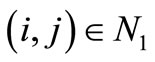 for which
 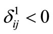 or some
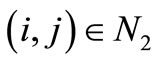 for which
  will enter the basis. Go to Step 2.
Step 5: Find the optimal value of 
5. Problem of the Manager of a Cell Phone Manufacturing Company
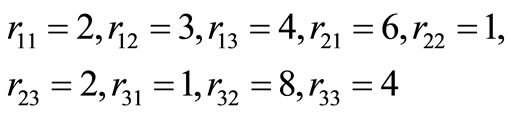
ABC company produces cell phones. These cell phones are manufactured in the factories (i) located at Haryana, Punjab and Chandigarh. After production, these cell phones are transported to main distribution centres (j) at Kolkata, Chennai and Mumbai. The cartage paid per cell phone is 2, 3 and 4 respectively when the goods are transported from Haryana to Kolkata, Chennai and Mumbai. Similarly, the cartage paid per cell phone when transported from Punjab to distribution centres at Kolkata, Chennai and Mumbai are 6, 1 and 2 respectively while the figures in case of transportation from Chandigarh is 1, 8 and 4 respectively. In addition to this, the company has to pay sales tax per cell phone. The sales tax paid per cell phone from Haryana to Kolkata, Chennai, Mumbai are 5, 9 and 9 respectively. The tax figures when the goods are transported from Punjab to Kolkata, Chennai and Mumbai are 4, 6 and 2 respectively. The sales tax paid per unit from Chandigarh to Kolkata, Chennai and Mumbai are 2, 1 and 1 respectively. The total public expenditure per unit when the goods are transported from Haryana to Kolkata, Chennai and Mumbai are 4, 2 and 1 respectively while the figures for Punjab are 3, 7 and 4. When the goods are transported from Chandigarh to distribution centres at Kolkata, Chennai and Mumbai, the total public expenditure per cell phone is 2, 9 and 4 respectively. Factory at Haryana can produce a minimum of 3 and a maximum of 30 cell phones in a month while the factory at Punjab can produce a minimum of 10 and a maximum of 40 cell phones in a month. Factory at Chandigarh can produce a minimum of 10 and a maximum of 50 cell phones in a month. The minimum and maximum monthly requirementof cell phones at Kolkata are 5 and 30 respectively while the figures for Chennai are 5 and 20 respectively and for Mumbai are 5 and 30 respectively. The bounds on the number of cell phones to be transported from Haryana to Kolkata, Chennai and Mumbai are (1, 10), (2, 10) and (0, 5) respectively. The bounds on the number of cell phones to be transported from Punjab to Kolkata, Chennai and Mumbai are (0, 15), (3, 15) and (1, 20) respectively. Thebounds on the number of cell phones to be transported from Chandigarh to Kolkata, Chennai and Mumbai are (0, 20), (0, 13) and (0, 25) respectively. The manager keeps the reserve stocks at the factories for emergencies, there by restricting the total transportation flow to 40 cell phones. He wishes to determine the number of cell phones to be shipped from each factory to different distribution centres in such a way that the total cartage plus the ratio of total sales tax paid to the total public expenditure per cell phone is minimum.
5.1. Solution
The problem of the manager can be formulated as a 3 × 3 linear plus linear fractional transportation problem (P1) with restricted flow as follows.
Let O1 and O2 and O3 denotes factories at Haryana, Punjab and Chandigarh. D1, D2 and D3are the distribution centres at Kolkata, Chennai and Mumbai respectively. Let the cartage be denoted by rij’s (i = 1, 2, 3 and j = 1, 2 and 3). The sales tax paid per cell phone when transported from factories (i) to distribution centres (j) is denoted by sij. The total public expenditure per cell phone for I = 1, 2 and 3 and j = 1, 2 and 3 is denoted by tij. Then


Let xij be the number of cell phones transported from the ith factory to the jth distribution centre.
Since factory at Haryana can produce a minimum of 3 and a maximum of 30 cell phones in a month, it can be formulated mathematically as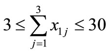 .
.
Similarly,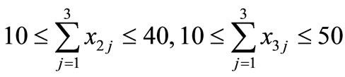 .
.
Since the minimum and maximum monthly requirement of cell phones at Kolkata are 5 and 30 respectivelyit can be formulated mathematically as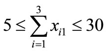 . Similarly,
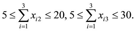
The restricted flow is P = 40.
The bounds on the number of cell phones transported can be formulated mathematically as


The above data can be represented in the form of Table 1 as follows.
Introduce a dummy source and a dummy destination in Table 1 with


and

and
 .
.
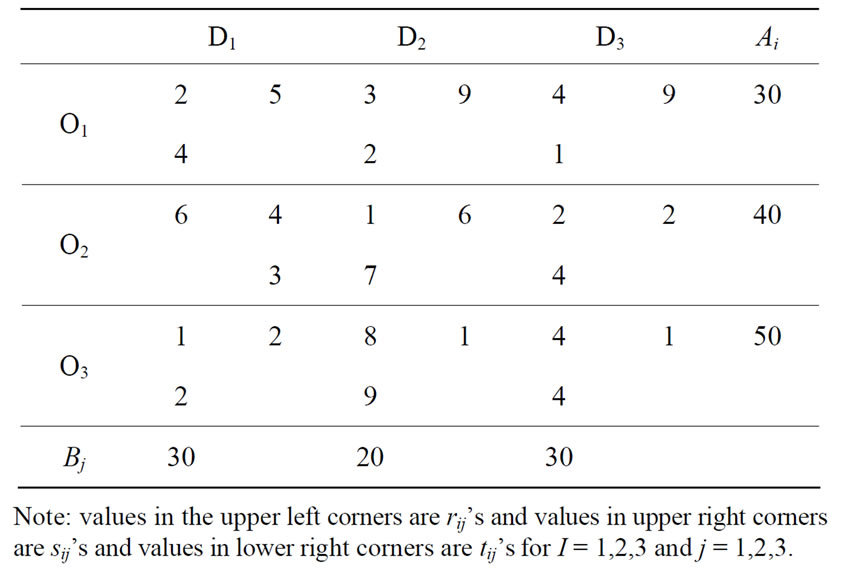
Table 1. Problem (P1).
Also we have

Now we find an initial basic feasible solution of problem (P2) which is given in Table 2 below.
Since  and
and  as shown in Table 3, the solution given in Table 2 is an optimal solution to problem (P2) and subsequently to (P1). Therefore
Therefore, the company should send 1 cell phone from Haryana to Kolkata, 2 units from Haryana to Chennai. The number of cell phones to be shipped from factory at Punjab to Chennai and Mumbai centres are 15 and 5

Table 2. A basic feasible solution of problem (P2).
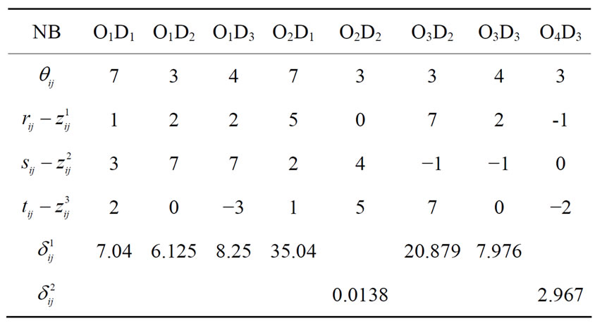
Table 3. Calculation of  and
and .
.
respectively. Factory at Chandigarh should send 17 units to Kolkata only. The total cartage paid is 50, total sales tax paid is 157 and total public expenditure is 167.
6. Conclusion
This paper deals with a linear plus linear fractional transportation problem where in the total transportation flow is restricted to a known specified level. A related transportation problem is formulated and it is shown that it exited an optimal solution. An algorithm is presented and tested by a real life example of a manufacturing company.
7. Acknowledgements
We are thankful to the referees for their valuable comments with the help of which we are able to present our paper in such a nice form.
References
[1] A. Gupta, S. Khanna and M. C. Puri, “A Paradox in Linear Fractional Transportation Problems with Mixed Constraints,” Optimization, Vol. 27, No. 4, 1993, pp. 375- 387. http://dx.doi.org/10.1080/02331939308843896
[2] M. Jain and P. K. Saksena, “Time Minimizing Transportation Problem with Fractional Bottleneck Objective Function,” Yugoslav Journal of Operations Research, Vol. 21, No. 2, 2011, pp. 1-16.
[3] F. Xie, Y. Jia and R. Jia, “Duration and Cost Optimization for Transportation Problem,” Advances in Information Sciences and Service Sciences, Vol. 4, No. 6, 2012, pp. 219-233. http://dx.doi.org/10.4156/aiss.vol4.issue6.26
[4] A. Khurana and S. R. Arora, “The Sum of a Linear and Linear Fractional Transportation Problem with Restricted and Enhanced Flow,” Journal of Interdisciplinary Mathematics, Vol. 9, No. 9, 2006, pp. 373-383. http://dx.doi.org/10.1080/09720502.2006.10700450
[5] K. Gupta and S. R. Arora, “Paradox in a Fractional Capacitated Transportation Problem,” International Journal of Research in IT, Management and Engineering, Vol. 2, No. 3, 2012, pp. 43-64.
[6] S. Misra and C. Das, “Solid Transportation Problem with Lower and Upper Bounds on Rim Conditions—A Note,” New Zealand Operational Research, Vol. 9, No. 2, 1981, pp. 137-140.
[7] S. Jain and N. Arya, “An Inverse Capacitated Transportation Problem,” IOSR Journal of Mathematics, Vol. 5, No. 4, 2013, pp. 24-27. http://dx.doi.org/10.9790/5728-0542427
[8] S. R. Arora and K. Gupta, “Restricted Flow in a NonLinear Capacitated Transportation Problem with Bounds on Rim Conditions,” International Journal of Management, IT and Engineering, Vol. 2, No. 5, 2012, pp. 226- 243.
[9] A. Khurana, D. Thirwani and S. R. Arora, “An Algorithm for Solving Fixed Charge Bi—Criterion Indefinite Quadratic Transportation Problem with Restricted Flow,” International Journal of Optimization: Theory, Methods and Applications, Vol. 1, No. 4, 2009, pp. 367-380.