American Journal of Operations Research
Vol. 2 No. 3 (2012) , Article ID: 22433 , 8 pages DOI:10.4236/ajor.2012.23045
Stochastic Programming Model for Discrete Lotsizing and Scheduling Problem on Parallel Machines
1Global Logistics, Kao Corporation, Tokyo, Japan
2Faculty of Business Administration, Toyo University, Tokyo, Japan
3Faculty of Social Systems Science, Chiba Institute of Technology, Chiba, Japan
4School of Creative Science and Engineering, Waseda University, Tokyo, Japan
Email: ishiwata.kensuke@kao.co.jp, jun@toyo.jp, shiina.takayuki@it-chiba.ac.jp, morito@waseda.jp
Received July 23, 2012; revised August 27, 2012; accepted September 7, 2012
Keywords: Stochastic Programming; Lotsizing and Scheduling; Parallel Machines; Scenario Aggregation Method
ABSTRACT
In recent years, it has been difficult for manufactures and suppliers to forecast demand from a market for a given product precisely. Therefore, it has become important for them to cope with fluctuations in demand. From this viewpoint, the problem of planning or scheduling in production systems can be regarded as a mathematical problem with stochastic elements. However, in many previous studies, such problems are formulated without stochastic factors, treating stochastic elements as deterministic variables or parameters. Stochastic programming incorporates such factors into the mathematical formulation. In the present paper, we consider a multi-product, discrete, lotsizing and scheduling problem on parallel machines with stochastic demands. Under certain assumptions, this problem can be formulated as a stochastic integer programming problem. We attempt to solve this problem by a scenario aggregation method proposed by Rockafellar and Wets. The results from computational experiments suggest that our approach is able to solve large-scale problems, and that, under the condition of uncertainty, incorporating stochastic elements into the model gives better results than formulating the problem as a deterministic model.
1. Study Background and Objective
In the manufacturing and supply chain industries in recent times, one of the most important challenges has been to determine how best to deal with the significant fluctuations in demand. Within the market environment of today, it is difficult to forecast customer behavior and not uncommon for any forecasts of demand that are made to miss the mark. As such, it has become necessary to take into account the element of uncertainty when developing plans. However, a challenge faced in production planning is the lot-scheduling problem. This stems from the fact that the main focus in production planning is on determination of lot sizes, which corresponds to tacticallevel decision-making, and determination of scheduling, which corresponds to operational-level decision-making, where the goal is to optimize both of these factors concurrently.
Almost all past research into the lot-scheduling problem has considered demand as a definite value. However, in light of the above-mentioned circumstances, it seems that in many cases, demand should be regarded as an uncertain element. For example, even if one is able to treat the most recent demand with certainty, it is quite likely that when decisions are made at a point in time later, uncertain elements will come into the mix. In such a situation, it becomes necessary to develop a plan which also takes into account those uncertain elements. Mathematical programming which takes these probabilistic factors into consideration is known as stochastic programming (Birge [1], Birge and Louveaux [2], Shiina [3]).
In the present study, we looked at a lot-scheduling problem on parallel machines and considered a stochastic programming model. Compared with a deterministic programming model that does not incorporate probabilistic factors, the stochastic programming model poses a large-scale problem for which it is often extremely difficult to find a solution. With this in mind, we felt it would be possible to obtain a solution by devising an approximate solution method based on the scenario aggregation method proposed by Rockafellar and Wets [4]. Specifically, we referred to the method of Løkketangen and Woodruff [5], which presents a specific general framework for problems incorporating 0 - 1 variables, to develop a procedure which provides an approximate solution.
We investigate the advantages of the stochastic programming model by numerical simulation to first compare the results obtained when following a deterministic programming model with the results obtained when the problem is considered in terms of a stochastic programming model, and we then assess the performance of the procedure. Next, we discuss the accuracy of the approximate solution and the computation time, and demonstrate the effectiveness of the solution method we developed.
2. Lot-Scheduling Problem
2.1. Definition of Problem
The lot-scheduling problem is to decide both the production lot size for each item type and the production time for each lot, in a lot production process in which preparatory work is required. In the present study, we consider a lot-scheduling problem on parallel machines. A summary of the problem is as follows.
Production is performed in which multiple types of items are exchanged around on multiple machines with differing performance that make up a single process. When the item types are exchanged, time and expense are required for preparatory work. Inventory storage costs arise in proportion to the amount of inventory. For each item type, an ordered shipping amount (demand quantity) is provided at designated times, and no item is allowed to run out. At any one time, a machine is capable of producing only one item type. The machines can be used only for a certain duration at a time, and it is necessary to carry out both preparation and production during that period. If the unit manufacturing cost is to be lowered and the lot size increased, then the expense incurred for storage of inventory increases; conversely, if the inventory is reduced, then preparatory work will need to be carried out more frequently, leading to the problem of increased time and expense for preparation.
2.2. Past Research and the Relevance of the Present Study
Past research into the lot-scheduling problem on parallel machines has, in many cases, studied deterministic programming models which treat customer demand as a definite value (for example, Meyr [6], Arai et al. [7]). So far, there has been almost no research into stochastic programming models for the lot-scheduling problem on parallel machines. Therefore, we assumed a situation in which some of the demand had to be treated as uncertain and formulated the lot-scheduling problem on parallel machines in terms of a stochastic programming model and then calculated a solution by applying the scenario aggregation method.
3. Formulation
3.1. Deterministic Programming Model
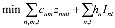
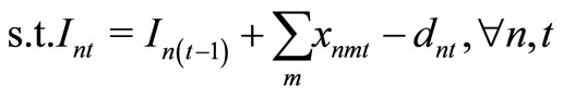
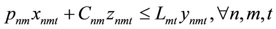
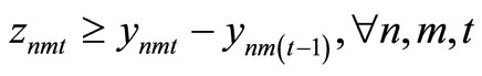
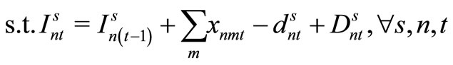
Item type, machine, and time are represented by N, M, and T, respectively. For the constants, the demand for item type n at time t is dnt, the length of time taken to create one unit of item type n on machine m is pnm, the length of time that machine m can be used at time t is Lmt, the cost of preparation for item type n on machine m is cnm, the time taken for preparation is Cnm, and the cost of storage of inventory for item type n is hn. For item type n on machine m at time t, the variable representing the production amount is xnmt, the variable indicating whether production is occurring is ynmt, and the variable indicating whether preparation is occurring is znmt. The variable representing the amount of inventory for item type n at time t is Int. The formulas used are as follows.
 (1)
(1)
 (2)
(2)
 (3)
(3)
 (4)
(4)
 (5)
(5)
 (6)
(6)
 (7)
(7)
 (8)
(8)
 (9)
(9)
 (10)
(10)
 (11)
(11)
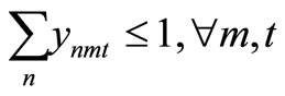
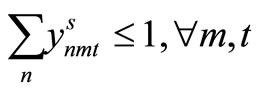
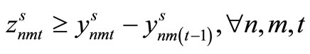
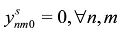
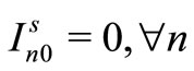
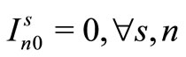
Here, (1) shows the objective function: the sum total of the preparation costs and the inventory storage costs; (2) updates the changes in inventory; (3) is the constraint on the time that a machine can be used; (4) reflects that, at each time, a machine is only capable of producing one type of item; (5) is a constraint on preparation being carried out; (6) and (7) are the initial conditions for production and inventory; and (8), (9), (10), and (11) are additional conditions on the individual variables.
3.2. Changes in Demand
In this section, we will discuss demand d, omitting the subscripted symbol for the item type. Specifically, this means that even though the item type is not indicated, the discussion assumes a specific item type.
Demand at time t,  , is defined as a stochastic variable, designated dt, which is assumed to follow a finite discrete distribution. The list of possible values for the stochastic variable across time T, represented d = (d1, ···, dT), is referred to as a scenario.
Based on the discrete and finite properties of the distribution, the number of scenarios is represented with the symbol S. The probability that a scenario s, that is to say , will occur is given by Ps (where
 ). In the scenario tree (the directed graph in Figure 1), the scenario is represented as routes from the root node to the leaf nodes.
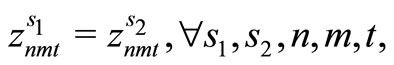
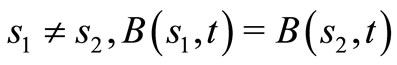
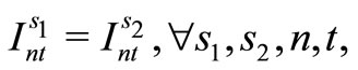
If the possible values for demand  and
and  of two scenarios s1 and s2 (with (s1 ≠ s2)) satisfy the equality
 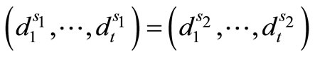 over the history to a certain time t, then they follow the same route on the tree, to time t.
The decision making for the two scenarios s1 and s2 must be the same to time t. At time t, the individual making decisions cannot anticipate that scenarios s1 and s2 will diverge in the future. This is because, at time t, they are not provided with information regarding the future development from time t + 1 onward, and they have to make a decision based on the history of dt until time t. This condition is referred to as the nonanticipativity condition.
The set of scenarios (represented as numbers)  can be partitioned into disjoint subsets at each time. The index set for scenarios equal to scenario s in history to time t is represented by
  and referred to as the scenario bundle. For example, in Figure 1, B(1, 1) = B(2, 1) = {1, 2}, and B(3, 1) = B(4, 1) = {3, 4}.
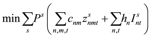
3.3. Stochastic Programming Model
The amount of demand for item type n at time t in scenario s is represented by  and the probability of occurrence of scenario s is Ps, as described above. Furthermore, the variable representing the production amount for item type n by machine m at time t in scenario s is
 , the variable indicating whether production is being carried out is
 , and the variable indicating whether preparation is being carried out is
 . The variable representing the amount of inventory of item type n at time t in scenario s is
 . The remaining symbols are as defined in Section 3.1. The relevant formulation is as follows.
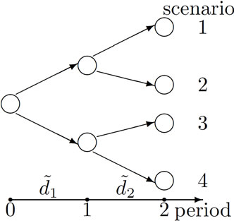
Figure 1. Scenario tree.
 (12)
(12)
 (13)
(13)
 (14)
(14)
 (15)
(15)
 (16)
(16)
 (17)
(17)
 (18)
(18)
 (19)
(19)
 (20)
(20)
 (21)
(21)
 (22)
(22)
 (23)
(23)
 (24)
(24)
 (25)
(25)
 (26)
(26)
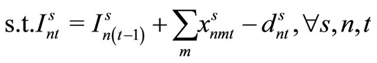
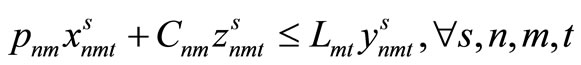
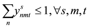
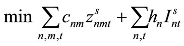
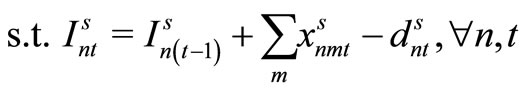
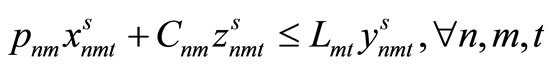
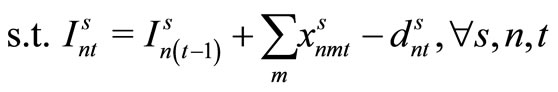
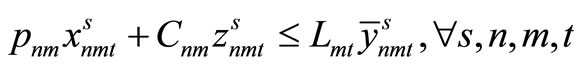
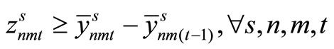
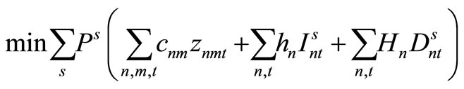
Here, (12) shows the objective function: the expectation of the sum total of the preparation costs and inventory storage costs; (13) updates the changes in inventory; (14)is the constraint on the time that a machine can be used; (15) reflects that, at each time, a machine is only capable of producing one type of item; (16) is a constraint on preparation being carried out; (17) and (18) are the initial conditions for production and inventory; (19), (20), (21), and (22) are the nonanticipativity conditions; and (23), (24), (25), and (26) are additional conditions on the individual variables.
4. Applying the Scenario Aggregation Method
4.1. Equivalent Deterministic Programming Problems
The formulation of problems (not only the lot-scheduling problem on parallel machines) via a stochastic programming model such as this poses a large-scale mathematical programming challenge, due to the variables that must be defined and the constraint conditions that must be listed for all of the scenarios. The lot-scheduling problem, which is modeled by the stochastic programming model considered in the present study, in particular, involves very substantial difficulties, if it is to be solved in its original format, as a mixed-integer programming problem. Therefore, in the present study, we took the problem structure arising from the modeling and formulation into account, and opted to pursue an approximate solution by using a framework known as the scenario aggregation method, which was proposed by Rockafellar and Wets [4].
4.2. Overview of the Scenario Aggregation Method
The scenario aggregation method is a solution method wherein a scenario sub-problem is defined for each route on the scenario tree leading from the root to a leaf, and the solutions obtained by solving the scenario sub-problems are aggregated. An overview of this solution method follows.
First, solutions are computed by solving the scenario sub-problems (we call these the admissible solutions). Next, the allowable solutions are aggregated, in order to compute a solution that satisfies the nonanticipativity condition (we call this the implementable solution).
The admissible solutions are guaranteed to be practicable for each scenario, but do not necessarily satisfy the nonanticipativity condition. In contrast, the implementable solution is guaranteed to satisfy the nonanticipativity condition, but is not guaranteed to be feasible for each scenario. Therefore, in the scenario aggregation method, the difference between these two types of solution is added to the scenario sub-problem in the form of a quadratic penalty term, and these differences are gradually allowed to converge until finally a solution to the problem to be solved can be computed.
The following section describes this process in detail.
4.3. Solution Algorithm
Below is described the specific procedure. In order to reduce the computation time required to reach the end condition in the scenario aggregation method, following the research of Løkketangen and Woodruff [5], we took into consideration only the convergence of integer variables, not the convergence of continuous variables.
Step 1
The following initial scenario sub-problem, corresponding to a scenario s, is solved and the admissible solutions  are computed.


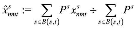
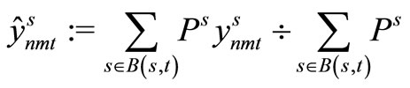
Step 2
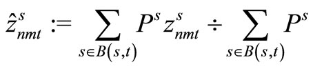
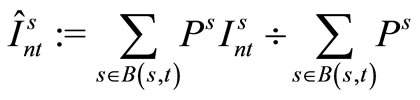
The following aggregation is applied to the admissible solutions, and the implementable solutions 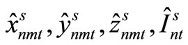 are computed. The values of the Lagrange multipliers
  are set to 0 and we go to Step 3.
Step 3
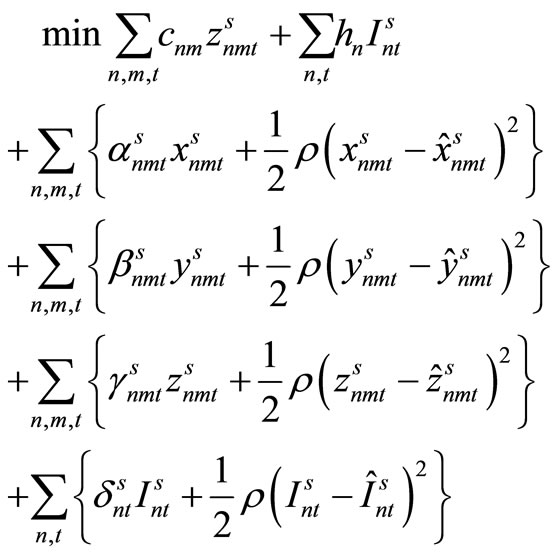
A scenario sub-problem that has the following 0-1 constraints, corresponding with each scenario s, is solved and the admissible solutions ,
,  ,
,  ,
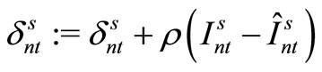
,  are computed. The objective function terms starting from the third term are penalty terms for the admissible and implementable solutions; ρ is a parameter in the scenario aggregation method.


Step 4
Aggregation is applied to the admissible solutions, and the implementable solutions ,
,  ,
,  ,
,  are computed. If the admissible solution
  and the implementable solution
  become equal, we go to Step 5. Otherwise, the values of the Lagrange multipliers
 ,
,  ,
,  ,
,  are altered using the equations below and we go to Step 3.
Step 5
The value of the converged integer variable  is substituted into the original problem formulation and the following linear programming problem is solved. The values of the continuous variables
 ,
,  ,
,  are computed to complete the procedure.


5. Numerical Experiments
5.1. Objective and Method of Numerical Experiments
Numerical experiments were performed based on the following perspectives.
1) The benefits of the stochastic programming model are assessed by comparison with the deterministic programming model (see Section 5.2).
2) Next, the behavior of the solution method using parameter ρ, as mentioned in Section 4.3, is analyzed. After that, the performance of the proposed solution method is assessed by comparing it with a case in which a direct branch-and-bound method-based solution method is used for the formulation of the stochastic programming model (a mixed-integer programming problem) (see Section 5.3).
The method of simulation was as follows. The numbers of item types N, machines M, and times T were set as (N, M, T) = (3, 2, 10), (3, 2, 15), (4, 2, 10), (4, 2, 15), (4, 3, 10), (4, 3, 15), (5, 3, 10), (5, 3, 15).
(These problems were then numbered from 1 to 8 so that problems could later be reference by number). Instances were then generated for each of these by random number. However, the changing demand scenarios were applied according to Table 1. In the table, up to eight of the T number of times have been divided into four equal sets, which are named P1, P2, P3, and P4 (for example, with T = 10, P1 represents t = 1, 2). The values in the table indicate the ratios of how the demand changes in
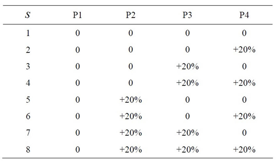
Table 1. Demand patern in each secenario.
each scenario, compared with the base amount of demand (the case where s = 1) when the changing demand scenarios were generated.
We consider cases with two, four, and eight scenarios. When S = 2, scenarios 1 and 2 each arise with a probability of ; when S = 4, scenarios 1, 2, 3 and 4 each arise with a probability of
 . The case when S = 8 is treated similarly.
The package used to apply the scenario aggregation method was OPL Studio 5.2. For optimization of the scenario sub-problem in Step 3, which is a quadratic programming problem having a 0 - 1 condition, and the mixed-integer programming problem used for comparison, the mixed integer optimizer in CPLEX (branchand-bound method-based solution) was used. The computer used for experiments was a DELL Precision 490 (Xeon 5060 3.20 GHz, memory 2 GB).
5.2. Value of Stochastic Solution
As a criterion of assessment, we used the value of stochastic solution (VSS) represented by the equation below. If we take the optimal objective function value of the stochastic programming model to be zp and the optimal objective function value of the deterministic programming model to be zd, then VSS is defined as follows.
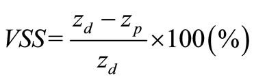
The demand at each time in the deterministic programming model was given by the mean of the demand across all scenarios in the stochastic programming model, and we assume that this demand will arise with probability 1 under that scenario only. Specifically, this was solved as one instance of the deterministic programming model, and the values of the decision variables were decided.
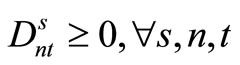
Next, we looked at the situation depicted in the formulation below that considers the penalty of running out of inventory, and computed the costs in each scenario when the values of the (only set of) decision variables xnmt, ynmt, znmt which could solve the current deterministic programming model were used (the number of results obtained corresponds with the number of scenarios). We then computed the mean of these results based on the probabilities of the scenarios arising and used this as the objective function of the deterministic programming model.  is the amount of demand which could not be satisfied by each scenario, and Hn is the penalty per unit of demand not satisfied (which corresponds to twice the inventory storage cost hn).
 (27)
(27)
 (28)
(28)
 (29)
(29)
 (30)
(30)
 (31)
(31)
Factors which do not appear in the original problem are considered here because, in contrast to conventional deterministic and stochastic programming models that do not allow for inventory to run out, when the values of variables are decided in a deterministic programming model that incorporates stochastic variation in the demand, it is possible for inventory to run out. As stated above, the penalty that arises when inventory runs out in such cases is assumed, in this numerical example, to be twice the inventory storage cost.
Table 2 lists the value of solutions from the stochastic programming model. Since it is necessary, in this case, to accurately assess the model, the formulation by the stochastic programming model (a mixed-integer program) was solved in its original format by the mixed integer optimizer in CPLEX, and only the data from which an optimal solution (within 3600 seconds) was obtained was considered. That is to say, the solution found at this time was not from the aforementioned scenario aggregation method. Table 2 shows the results for Problem 1 and Problem 5, for which optimal solutions could be obtained for all scenarios (as shown in the table).
From Table 2, it is apparent that when the number of scenarios increases, the VSS value increases accordingly. This is thought to be due to the fact that when the number of scenarios increases and the element of uncertainty
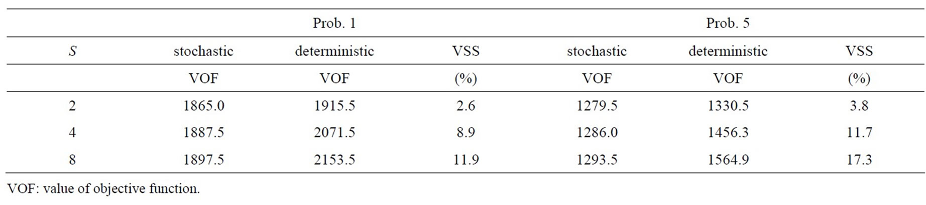
Table 2. Value of solutions from the stochastic model.
grows, the benefit of the stochastic programming model also increases.
In this section, we have shown only the case solvable as an integer programming problem that is equivalent to the stochastic programming model. However, in general, the scale of the problem grows as the number of scenarios is increased, making it more difficult to obtain a good solution (the optimal solution or one close to the optimal solution). As such, the importance of a procedure for finding the solution for a stochastic programming model directly and in a short period of time is heightened.
5.3. Assessment of Performance of the Proposed Solution Method
The optimal objective function values and computation times for the solution method proposed in the present study and the method of using the mixed integer optimizer in CPLEX directly to determine the formulation of the stochastic programming model (this will be referred to below simply as mixed-integer programming) were compared for the problem groups described in Section 5.1 for two, four, and eight scenarios.
The computation time for the solution method of the present study and mixed-integer programming were both limited to less than 3600 seconds; if the optimal value was not obtained by mixed-integer programming, a tentative objective function value was computed when the computation time reached the limit. The results are shown in Tables 3-5.
With proposed solution method, it was necessary to set the value of the parameter ρ that appears in Step 3 of Section 4.3. It was predicted that the behavior of the optimization would depend on this parameter value. Therefore, all of the results are shown for the values ρ = 0.2, 0.4, 0.6, 0.8, and 1.0. The optimization problems that appear in each step of the proposed solution method, as described in Section 4.3, were solved by using CPLEX as stated above.
Two points are of interest here:
• The relationship between the parameter set and the behavior of the solution method
• The performance of the proposed solution method in contrast to the case where the mixed-integer programming problem was solved directly using the branch-and-bound method-based solution
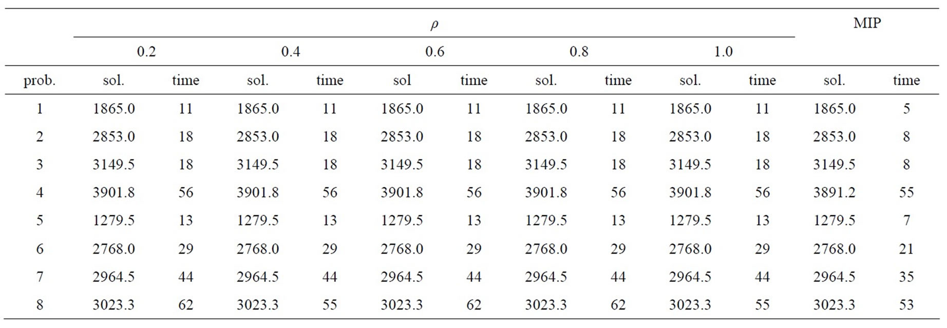
Table 3. Results from the stochastic model (# of scenario = 2).
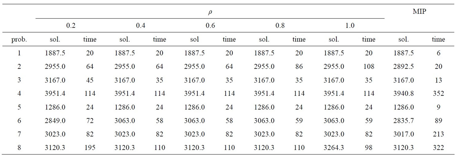
Table 4. Results from the stochastic model (# of scenario = 4).
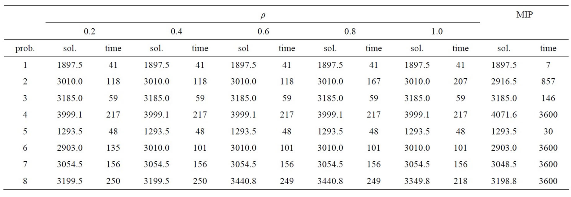
Table 5. Results from the stochastic model (# of scenario = 8).
The changes in behavior that result from changing the parameter ρ can be observed by comparing within a given row of a particular table. However, no specific pattern of behavior can necessarily be observed in the computation times and the optimal objective function values, and even when the parameter is changed in addressing the same problem, one cannot say that the effect is large enough to bring about any significant differences.
Comparing the solution method proposed in the present study and mixed-integer programming using Tables 3-5 reveals that although the proposed solution method does not always compute the same result as mixed-integer programming, in many cases either the same or an extremely close value is obtained.
There is a striking increase in the computation time of mixed-integer programming as the number of scenarios increases. In contrast, the computation time of the solution method we propose is relatively short, and although it falls a little behind the results of the latter in terms of how good the solution is, in cases where there are many scenarios, it is overwhelmingly superior in computation time. In particular, when the number of scenarios is high (S = 8), the proposed solution method obtains the feasible solution in a short period of time, in contrast to the mixed-integer programming computation, which frequently reaches the upper limit of time and has to stop.
This difference in computation time trends is thought to be due to the fact that, with the solution method we propose, although the computation time grows as the number of scenarios increases, the fact that the problem is broken down into sub-problems for each scenario which are then solved means that the effects of increasing the number of scenarios can be limited, compared to mixed-integer programming.
6. Conclusion and Future Challenges
In the present study, we considered the formulation of the lot-scheduling problem on parallel machines using a stochastic programming model and demonstrated the benefit of such a model over a deterministic programming model.
We developed an approximate solution method which applied the scenario aggregation method and demonstrated that even when the number of scenarios increases, thus making the problem large in scale, it is possible to compute an accurate solution that is of practical application in a short period of time.
REFERENCES
- J. R. Birge, “Stochastic Programming Computation and Applications,” INFORMS Journal on Computing, Vol. 9, No. 2, 1997, pp. 111-133. doi:10.1287/ijoc.9.2.111
- J. R. Birge and F. Louveaux, “Introduction to Stochastic Programming,” Springer-Verlag, Berlin, 1997.
- T. Shiina, “Stochastic Programming (in Japanese),” In: M. Kubo, A. Tamura and T. Matsui, Eds., Ôyô Sûri-Keikaku Handbook, Asakura Syoten, Tokyo, 2002, pp. 710-769.
- R. T. Rockafellar and R. J.-B. Wets, “Scenarios and Policy Aggregation in Optimization under Uncertainty,” Mathematics of Operations Research, Vol. 16, No. 1, 1991, pp. 119-147. doi:10.1287/moor.16.1.119
- A. Løkketangen and D. L. Woodruff, “Progressive Hedging and Tabu Search Applied to Mixed Integer (0,1) Multistage Stochastic Programming,” Journal of Heuristics, Vol. 2, 1996, pp. 111-128.
- H. Meyr, “Simultaneous Lotsizing and Scheduling on Parallel Machines,” European Journal of Operational Research, Vol. 139, No. 2, 2002, pp. 277-292. doi:10.1016/S0377-2217(01)00373-3
- H. Arai, S. Morito and J. Imaizumi, “A Column Generation Approachfor Discrete Lotsizing and Scheduling Problem on Identical Parallel Machines,” Journal of Japan Industrial Management Association, Vol. 55, 2004, pp. 69-76.