American Journal of Operations Research
Vol. 2 No. 1 (2012) , Article ID: 17837 , 16 pages DOI:10.4236/ajor.2012.21013
Optimal Ordering Policy of Deteriorating Items with Mixed Cargo Transportation over a Finite Planning Horizon
Department of Industrial Engineering & Management, National Chaio Tung University, Hsinchu, Chinese Taipei
Email: hsimei@cc.nctu.edu.tw, yahuilin2@ydu.edu.tw
Received January 21, 2012; revised February 27, 2012; accepted March 8, 2012
Keywords: Transportation Costs; Deteriorating Items; Inventory Management
ABSTRACT
In this paper, we propose a deteriorating items inventory model with constant demand and deterioration rates, and mixed cargo transportation modes. The transportation modes are full container load (FCL) and less than container load (LCL). Deteriorating items, such as specialty gases which are applied in semiconductor fabrication, deteriorate owing to environmental variation. Exact algorithms are proposed to determine the optimal inventory policies over a finite and an infinite planning horizon. Numerical examples are given to illustrate the proposed solution procedures. In addition, when the deterioration rate is large, the results of the proposed model perform better compared to the inventory model proposed by Rieksts and Ventura (2008).
1. Introduction
In this paper, we study a deteriorating items inventory model with mixed cargo transportation (full container load, FCL, and less than container load, LCL) over a given finite planning horizon. The customer’s demand per unit time d is constant and shortage is not allowed. The retailer places orders to its supplier and goods are transported by cargos. FCL and LCL cargoes are used. LCL is a shipment of cargo by which goods do not fully fill the container. The remaining space of the Less than Container may be filled with goods of other shippers. Generally, the transportation cost per unit under FCL is cheaper than LCL. Therefore, if goods can fill an entire container, FCL cargo will be the first choice.
In this paper, the assumptions are as follows: 1) supplier capacity is unlimited; 2) the delivery time is constant; 3) the salvage of inventory is zero; 4) the retailer needs to satisfy customers’ demand and shortage is not allowed. The retailer intends to determine the optimal order interval in order to minimize the total cost.
in Taiwan region’s semiconductor fabrication industries, many manufacturers need to import raw materials from abroad, such as certain specialty gases which may deteriorate owing to environmental variation. This research is motivated by a gas importing company from Taiwan region. The gas importing company makes gas supply contracts with customers for a certain time period, and the contracts indicate that the retailers shall supply raw materials to meet customers’ demands within a given time period. FCL and LCL are allowed. For example, Company A is the top supplier of electronic specialty gases in Taiwan region, and its’ customers include many international semiconductor manufacturing companies. Company A also provides the on-site gas generation system that includes small membrane cabinets, packaged plants, large air separation and hydrogen/carbon monoxide plants and industrial gas pipelines. Generated Gas Systems benefit customers by not only providing economical gas supply but also creating environmental advantages through reduced truck deliveries. In the gas generation system, since gas leakage cannot be completely prevented or avoided owing to miss operation or gas pipeline deterioration and failure, the gas monitoring system is built to detect the amount of gas leakage. In addition, Company A has signed supply contracts with various semiconductor manufacturing companies to supply various types of bulk gas, bulk specialty gas, and electronic chemicals. Under these contracts, Company A is obliged to supply gas to meet customers’ demand ( ) within a finite horizon
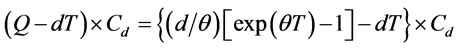
  and shortage is not allowed. However, Company A needs to order gas from foreign suppliers in order to satisfy customers’ demand for bulk gas, bulk specialty gas, and electronic chemicals. In addition to a fixed ordering cost (K), each order payment also includes fees related to the quantity of transportation containers and the number of items of LCL shipping.
After the termination of the contract, the surplus inventory still belongs to Company A and customers only need to pay for the quantity which they have used. Since surplus inventory of industrial gas in the on-site gas generation system may be disposed with additional costs, Company A therefore expects to reserve no surplus product after the termination of the contract. According to the above-mentioned situation, Company A should construct its own inventory model so as to determine the optimal order interval.
In this paper, we refer to Company A as retailer. We develop a deteriorating items inventory model with mixed cargo transportation to determine the order interval of goods over a given finite planning horizon. The model is formulated to minimize the retailer’s expected cost. The following costs are considered. 1) The deteriorating costs of gas : the percentage of gas which has deteriorated per unit time is
 . The purchase cost per unit of gas multiplying by the deterioration rate
  equals to
 ; 2) Holding cost h per unit time: the holding cost per unit is the sum of interest, insurance and the holding cost; 3) Setup cost K per order; 4) Transportation cost: two kinds of transportation costs are considered. The first one is FCL cost which is calculated based on the number of containers used multiplying by the container fee per unit
 . The other one is LCL cost.
Then we define the conditions for the existence of the optimal solution and develop a procedure to determine the optimal order interval. The rest of this paper is organized as follows: The assumptions and notations for the proposed model, the optimal ordering model and the solution procedure are proposed in Section 3. Some numerical examples are performed in Section 4. Finally, conclusions and future study are stated in Section 5.
2. Literature Review
In this paper, we propose the deteriorating items inventory model to determine the optimal order interval over the finite planning horizon. The retailer can receive goods with mixed cargo transportation (FCL and LCL). Nowadays mixed cargo is commonly used in international air or sea cargo shipping industry. The deteriorateing items inventory model with mixed cargo transportation (FCL and LCL) in this paper fall into the categories: 1) continuous review inventory problem with bi-modal transportation cost (Rieksts and Ventura [1]); 2) deteriorating items inventory model with deterministic demand and fixed lifetime (Goyal & Giri [2], Li et al. [3]). Bimodal transportation problem discussed by Rieksts and Ventura [1] is truckload (TL) transportation and less than truckload (LTL). In fact, the inventory problem of the mixed cargo and bi-modal transportation cost are identical except that vehicles used. In TL and LTL, the vehicle is a truck but the vehicle becomes a container in our study. Thus, this paper reviewed recent studies of 1) continuous review inventory problem with bi-modal transportation cost; and 2) deteriorating items inventory model with deterministic demand and fixed lifetime.
Rieksts and Ventura [4] classified continuous review inventory models with bi-modal transportation cost as four types. The first type is TL with no freight discount. TL with no freight discount is that the cost per load does not change with the number of truckloads (Aucamp [5] and Lippman [6]). The second type is TL with quantity or freight discount, TL with quantity or freight discount is TL shipments with discounts on the cost per load or quantity as the number of truckloads increase (Lee [7], Hwang et al. [8], Tersine et al. [9]). The third type is TL and LTL with no freight discount. TL and LTL inventory models are discussed and compared simultaneously in this category (Adelwahab and Sargious [10]), Swenseth and Godfrey [11], Rieksts and Ventura [1]). The Fourth type is TL with other delivery. TL with other delivery is TL and LTL inventory models with the other options of delivery (e.g. shipping to each retailer directly or peddling deliveries to a customer (Burns et al. [12]), the shipment from origin, in-transit to the destination (Larson [13])).
Two extensive survey papers on deteriorating items inventory models have been published by Goyal & Giri [2] and Li et al. [3]. Studies of deteriorating items inventory model with deterministic demand fixed lifetime are discussed respectively as follows; 1) deteriorating items inventory model with deterministic demand: Li et al. [3] classified deteriorating items inventory model with deterministic demand as five types of demand: fixed demand rate (Chung and Lin [14], Benkherouf et al. [15]), uniform demand (Heng et al. [16], Raafft et al. [17], Goh et al. [18]), time-varing demand (Yan and Cheng [19], Giri et al. [20], Teng et al. [21]), stock-dependent demand (Chung et al. [22], Giri and Chaudhuri [23], Bhattachaya [24], Wu et al. [25]) and price-depend demand (Wee [26], Wee and Law [27]); 2) deteriorating items inventory model with fixed lifetime: Li et al. [3] classified deteriorating items inventory model with fixed lifetime as two deteriorating rates: a constant deteriorating rate (Ghare and Schrader [28], Shah and Jaiswal [29], Padmanabhana and Vratb [30], Bhunia and Maiti [31]) and time-varing deteriorating rate (Bhunia and Maiti [32], Abad [33], Mukhopadhyay et al. [34], Mahapatra [35]).
The inventory models with a bi-modal transportation cost proposed by Rieksts and Ventura [1] is closely related to our problem. In this paper, we develop a more general deteriorating items inventory model with mixed cargo transportation to determine the optimal order interval, and the model of Rieksts and Ventura [1] is a subset of the proposed model. Under proposed model, the two types of transportation costs and the deteriorating cost of goods are formulated respectively in the deteriorating items inventory model to decide the optimal order interval.
3. Problem Formulation
3.1. Notations
The related notations are given as follows:
 : integer operator, integer value equal or greater than x.
 : integer operator, integer value equal or less than x.
 : the constant deterioration rate of a unit gas volume per unit time, where
 .
.
 : the unit deteriorated cost per unit gas volume per unit time,
 .
.
 : on hand inventory at time t.
 : demand rate is constant and known.
 : holding cost per unit item per unit time.
 : period of the whole planning horizon.
 : order times during the entire period
 .
.
 : set up cost per order;
 .
.
 : the unit container cost.
 : shipping cost of LTL per unit item.
 : the order quantity per cycle.
 : container maximum capacity.
 : the total transportation cost per cycle.
 : the consumption duration for
  that includes real demand and deteriorated items,
 .
.
Decision variables:
 : order interval.
Intermediate variables:
 : the space defined by
 : the decision space defined by
 : optimal order interval in
  over infinite planning horizon.
 : optimal order interval in
  over infinite planning horizon.
3.2. Problem Assumptions and Formulation
3.2.1. Infinite Planning Horizon Model
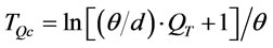
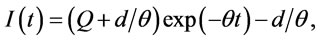
The mathematical model is formulated to determine the order interval with mixed cargo transportation for minimizing retailer’s total cost. The customer’s demand is a constant rate of d units per unit time. The inventory deterioration rate  is the percentage of a unit gas volume deteriorated per unit time. Therefore the inventory level will decrease owing to customer’s demand and gas deterioration. Thus, the differential equation representing the inventory status (Ghare and Schrader [28]) is given by:

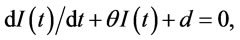 (1)
(1)
with the boundary condition  and
and . The solution of (1) is:

 (2)
(2)
The order quantity per cycle can be written as:
 , (3)
, (3)
where T is the order interval. For ignorance of lead time and impermissible shortage, the optimal ordering policy is to place order when the inventory level is zero (zero inventory policy). Under the zero inventory policy to determine order quantity Q is equivalent to determine the order interval T, i.e., order quantity Q is equal to  plus total deteriorating quantities per cycle. Now we will formulate the retailer’s total cost function per cycle, denoted as
 , and determine the optimal order interval
  for infinite planning horizon.
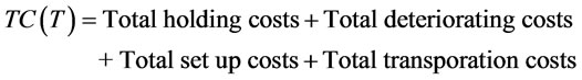
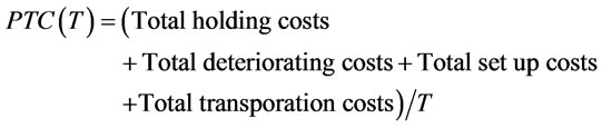
The items considered in  are total holding costs, total deteriorating costs, total set up costs and total transportation costs. The total cost function per unit time, denoted as
 , is given as follows:
 (4)
(4)
 (5)
(5)
The relevant items in (4) are formulated respectively as follows:
1) Total holding cost per cycle
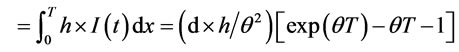 (6)
(6)
2) Total deteriorating costs per cycle: total deteriorateing quantities per cycle is  and total deteriorated costs is
 . By (3), we get
 (7)
(7)
3) Total set up costs per cycle is K.
4) Total transportation costs per cycle:
 (8)
(8)
Because the unit item transportation cost with FCL is cheaper than it with LCL transportation, therefore FCL cargo is used first when order quantity Q is larger than a container maximum capacity . The remaining goods are defined as
  that will be transported by LCL or FCL. Goods transportation cost with FCL is charged by the amount of a container fee multiplied by total numbers of container used. Goods transportation cost with LCL is charged by unit transportation fee
  multiplied by remaining quantities. We assume
  >
> .
.
Now we will discuss the relationships between T and .
.  is the consumption length for quantity
  that includes real demand plus deteriorated items. The relationship between
  and
and  is defined as follows by (3).
 . (9)
. (9)
Then  is:
is:
 (10)
(10)
The numbers of FCL cargo used per cycle is between  and
and , i.e.,
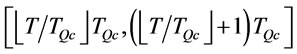
 . (11)
In other words, the order interval T is between  and
and , i.e.,
 (12)
(12)
If  is not an integer, then we must consider whether the remainder will be transported by FCL or LCL. The remaining quantities is equal to
  that will be transported with LCL when
  is less than or equal to
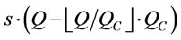 , otherwise that will be transported with FCL. By (3) the remaining quantities
 are also equal to
 .
.
Therefore the remainder transportation cost is considered as follows:
 . (13)
Then the total transportation cost per cycle  is:
is:
 (14)
(14)
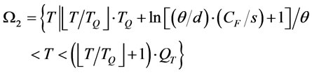
Let
 then
then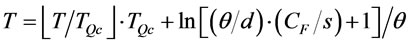 . Therefore we define
 (15)
(15)
and
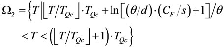 (16)
(16)
In , the transportation cost of remainders with LCL is cheaper than that with a full cargo. In
 , remainders are transported with FCL.
Hence  can be reformulated as follows:
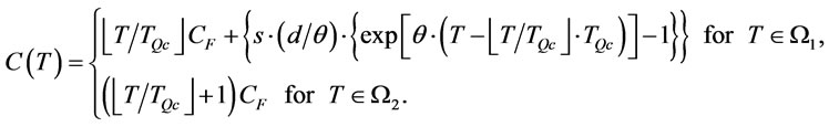 (17)
(17)
Substituting (6)-(17) into (5), the inventory problem over infinite planning horizon can be converted to problem A as follows:
(Problem A)
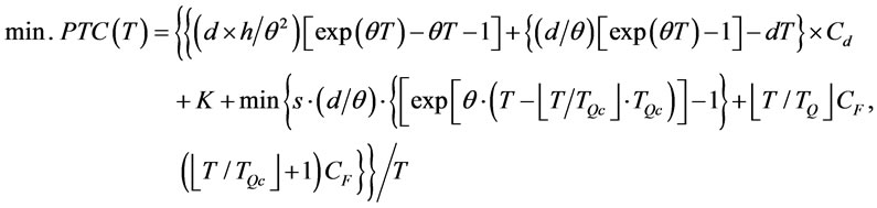 (18)
(18)
subject to .
.
We reformulate  on space
  and
and  respectively as follows:
 (19)
(19)
and
 (20)
(20)
After formulating the inventory problem over infinite planning horizon, in the following section, we will discuss about this problem over finite planning horizon.
3.2.2. Finite Planning Horizon Model
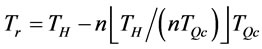
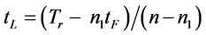
Suppose the finite planning horizon denote as . We assume the total order times is
  in
in  and the corresponding order intervals are
 , respectively. Given the total cost of the whole planning horizon
  is denoted as
 . Thus the inventory problem over finite planning horizon is formulated as follows:
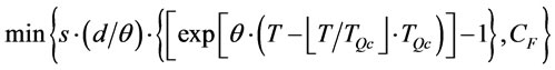
(Problem B)
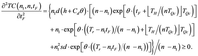
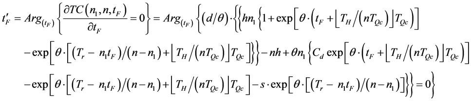
min. (21)
(21)
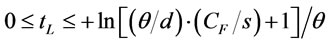
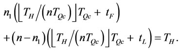
subject to , and
, and ,
, .
.
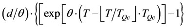
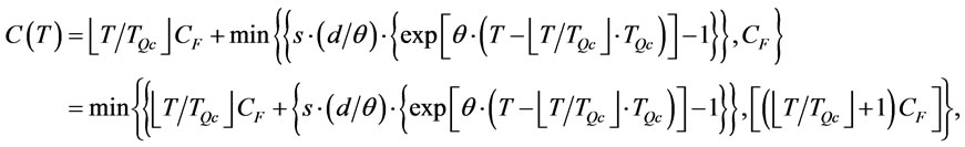
Where  is the total cost occurred in
 , and according to (18),
  can be expressed as follows.
 . (22)
and
 (23)
(23)
In problem B, we must find the optimal values of n and  to minimize
 .
.
3.3. Optimal Ordering Policy
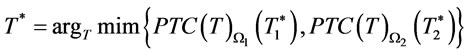
3.3.1. Optimal Ordering Policy over the Infinite Planning Horizon
We first prove that the optimal ordering policies for infinite and finite planning horizon problems as shown in (18) and (21) will satisfy the zero inventory policy in proposition 1.
Proposition 1. The optimal ordering policy for equation (18) and (21) will satisfy the zero inventory policy.
Proof. See appendix A.
We will show  and
and 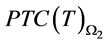 are both convex functions in proposition 2. Then we can determine optimal order interval
  and
and  for the two spaces respectively.
Proposition 2. For a given ,
,  and
and  are convex functions, i.e.,
 and
and .
.
Proof. See appendix B.
Proposition 3. For a given , there exist a
and a  such that
  and
and  for the two spaces respectively, where
 (24)
(24)
and
 (25)
(25)
However, when  or
or  is not in its spaces, in such condition, we will consider the end points to replace
  or
or .
.
Proof. See appendix C.
In proposition 2 and 3,  is assumed known.
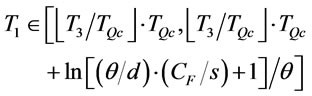
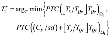
In order to find the optimal value  for minimizing
 in problem A, we first determine the optimal order interval without considering the transportation cost item (
 ) in
) in , denoted as
  by proposition 4. Then with proposition 5 we show
  is in the interval
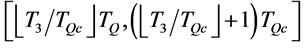 .
.
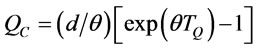
Proposition 4. Let there exist a
  such that
 , where
 (26)
(26)
Proof. See appendix D.
Proposition 5. The optimal order interval  for problem A is in the interval
 .
.
Proof. See appendix E.
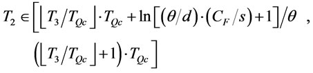
By Proposition 5, . The interval
 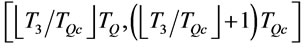 is divided into
  and
and  as shown in (15) and (16). By proposition 2 and 3, we obtain the optimal values of
  and
and  respectively. Proposition 6 is provided to find optimal order interval
  for problem A.
Proposition 6. There exists an optimal order interval  in problem A, and
  is determined by the following procedure:
Step 1: Find  by proposition 4, then let
 .
.
Step 2: Find  by proposition 3. If
then set  by proposition 2 and 3, and go to step 4. Otherwise, go to step 3.
Step 3: Compare  for the two end points. Set
and go to step 4.
Step 4: Find  by proposition 3. If
then set  by proposition 2 and 3, and go to step 6. Otherwise, go to step 5.
Step 5: Compare  for the two end points. Set
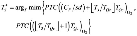
and go to step 6.
Step 6: Optimal order interval
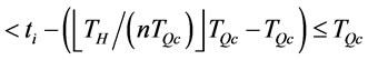
3.3.2. Optimal Ordering Policy over the Finite Planning Horizon
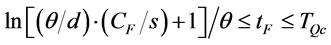
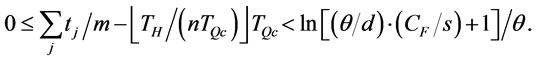
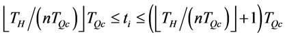
We first determine the upper bound of optimal order times  by Proposition 7.
Proposition 7. The optimal order times  over finite planning horizon is at most
Proof. See appendix F.
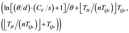
By proposition 7, the upper bound of order times n is 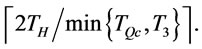 Proposition 8 and 9 will show the order intervals over finite planning horizon in the optimal order policy may not be equal, and the difference between any two order intervals is not more than
 . We also find the lower and upper bounds for the order intervals.
Proposition 8. Let  and
and  be any two order intervals in the optimal ordering policy, then
 .
.
Proof. See appendix G.
Proposition 9. Any order interval  in the optimal ordering policy over finite planning horizon is satisfied
 .
.
Proof. See appendix H.
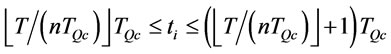
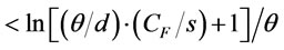
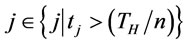
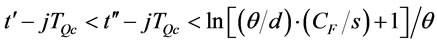
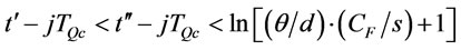
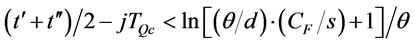
Proposition 9 shows the lower bound of any order interval in optimal ordering policy is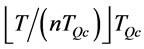 . Based on proposition 8 and 9, Proposition 10 will show that order intervals in the optimal ordering policy have at most two types.
Proposition 10. Under the given order times n, we know the order intervals in the optimal ordering policy have at most two types, 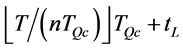 where
where

and 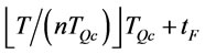 where
where
 .
.
Proof. See appendix I.
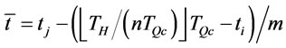
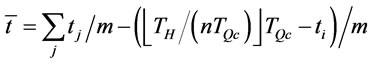
Based on proposition 8, 9 and 10, we assume that there are  (
( ) order times with order interval length
 and
and  order times with order interval length
  over finite planning horizon
  i.e.,
i.e.,
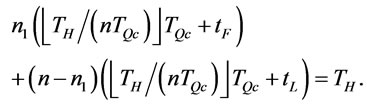 (27)
(27)
Therefore  can be denoted as
 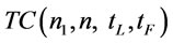 , and the problem B can be converted to problem B1 as follows:
(Problem B1)
 (28)
(28)
subject to
 ,
,
 ,
,
In problem B1, we let
 , (29)
then  in problem B1 can expressed as a function of
  as follows:
 . (30)
Therefore  can be denoted as
  , and problem B1 can be transformed to problem B2 as follows:
(Problem B2)
 (31)
(31)
subject to
 .
.
In Problem B2, the two constraints about  are combined as follows.
 (32)
(32)
i.e.,
 . (33)
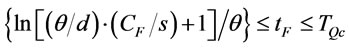
In (33), if

is larger than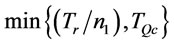 , then problem B2 has no feasible solution.
By proposition 11, we will show 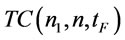 in problem B2 is a convex function. Then we can determine
  to find the optimal cost in problem B2.
Proposition 11. For a given  and n,
  is a convex function, i.e.,
  , and there exist a
  such that
 , where
 (34)
(34)
Proof. See appendix J.
Given n and , we get
  by proposition 11, but
  may not satisfy (32), i.e., the optimal order interval
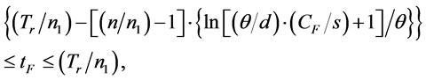
  will be considered the two end points of (32). Therefore an algorithm in proposition 12 is provided to find the optimal ordering policy over finite planning horizon.
Proposition 12. The optimal ordering policy over finite planning horizon is determined by the following procedure:
Step 0: Initialize ,
,  ,
,  and
and . Calculate
 ,
,  (by proposition 4) and
  (by proposition 7), let n = 1 and n1 = 0. Go to step 1.
Step 1: Set , find the lower bound L and upper bound U of
  as follows:
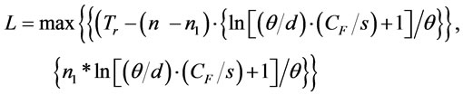
and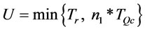 . Go to step 2.
Step 2: Check whether  is satisfied. If
  is hold, go to step 3, otherwise go to step 5.
Step 3: Find  by proposition 11. If
  is not in the interval [L, U] then we consider two conditions 1) if
 , let
, let ; 1)
; 1) , let
, let . Go to step 4.
Step 4: Calculate . If
. If , then set
 ,
,  ,
,  ,
, . Go to step 5.
Step 5: If , set
, set  and go to step 2, otherwise go to step 6.
Step 6: If , set
, set  and
and . Go to step 2, otherwise go to step 7.
Step 7: Print ,
,  ,
,  and
and .
.
The optimal ordering policy is as follows:
There are  order times where
  order times with order interval length
  and
and  order times with order interval
 , where
 , the optimal cost is
 .
.
4. Computational Study
With two examples given by Rieksts and Ventura [1], we demonstrate our proposed solution procedures for infinite and finite planning horizons with considering deteriorateing item. We will show that the approach proposed by Rieksts and Ventura cannot be applied to deteriorating items. The results for each example are also shown in Table 1.
Example 1a. (Infinite planning horizon) Suppose the customer demand rate (d) =2 units/month, and and the other relevant parameters are given as follows: container maximum capacity ( ) is 20 unit, holding cost (h) = $ 1/unit/month, set up cost per order (K) = 200/per order, unit container fee (
 ) = $60.2/unit, and goods transportation cost with LCL (s) is charge by $3.75/unit per unit good. (The infinite example in [1]).
Example 1b. Data are given by Example 1a, and additional data are given as follows: the deterioration rate ( ) is 0.05 and the unit deteriorated cost per unit gas volume per unit month (
 ) is $ 0.5/unit/month.
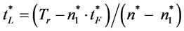
With our proposed solution procedure stated in proposition 6, in step 1 we find that  = 11.484 by proposition 4 and
  =1. In step 2, we find that
  = 11.1749 by proposition 3, and
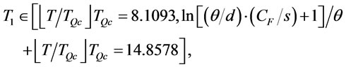
we set  = 11.1749 and go to step 4. In step 4, we find that
  = 13.9267 by proposition 3 and

then we go to step 5. In step 5, we compare  for the two end points in
  and set
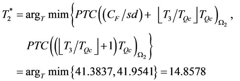
then we go to step 6. In step 6, optimal order interval
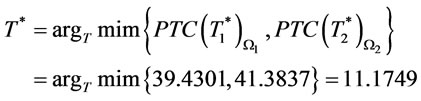
and optimal total cost per month is 39.4301.
Example 2a. (finite planning horizon) Suppose the customer demand rate (d) = 1 units/month, period of the whole planning horizon ( ) = 5 month and the other relevant parameters are given as follows: container maximum capacity (
 ) is 4 unit, holding cost (h) = $2/unit/month, set up cost per order (K) = 25/per order, unit container fee (
 ) = $1000/unit, and goods transportation cost with LCL (s) is charge by $500/unit per unit good. (The finite example in [1])
Example 2b. Data are given by Example 1a, and additional data are given as follows: the deterioration rate ( ) is 0.2 and the unit deteriorated cost per unit gas volume per unit time (
 ) is $0.5/unit/ month.
With our proposed solution procedure in proposition 12, in step 0, initialize  = 0,
= 0,  = 1,
= 1,  = 0,
= 0,  , let n = 1 and
  = 0. And we find that
 ,
,  = 3.95019 and
  = 4 by proposition 4 and 7, then we go to step 1. In step 1, set
  2.06107, we find
  and
and

then go to step 2. In step 2, L > U, we go to step 5. In step 5,  , let
, let  and go to step 1. In step 1,
  = 2.06107 and L = U = 2.06017. Go to step 2. In step 2, L = U, go to step 3. In step 3, we find
  by proposition 11, let
  = 2.06107. Go to step 4. In step 4, calculate
  and
and ,
,  ,
,  ,
,  and
and . Go to step 5. In step 5,
  , go to step 6. In step 6,
  and set n = 2 and go to step 1. We repeat the algorithm until
 . At the termination of algorithm, we find
 ,
,  ,
,  and
and , i.e., The optimal ordering policy is: there are 1 order times with order interval length 5 over finite planning horizon
  = 5 and optimal total cost is 2062.71.
From Table 1, we know when the deterioration rate ( ) approach to zero, our results are identical to those obtained by Rieksts and Ventura’s model. However in the scenario with considering deteriorating item, Rieksts and Ventura’s model is not work well.
In Figure 1 we show the differences of costs per unit time between the two infinite models which increase with the increased value of the deterioration rate ( ). Similarly, Figure 2 shows the cost differences between the two finite models which increase with the increased value of the deterioration rate (
 ). When the deterioration rate (
 ) is large, Rieksts and Ventura’s model does not work well. However, the proposed model can obtain the optimal cost.
5. Conclusion
In this paper we propose approaches to resolving the problems of the deteriorating items inventory model with mixed cargo transportation (FCL and LCL) to determine the optimal order interval and to minimize the cost per unit and the total cost over infinite and finite planning horizon. The optimal order intervals over infinite and finite planning horizons are derived and the solution procedures are proposed. Numerical examples are also illustrated. From example, when the deterioration rate ( ) approaches to zero, our results are identical to those obtained from Rieksts and Ventura’s model. The differences
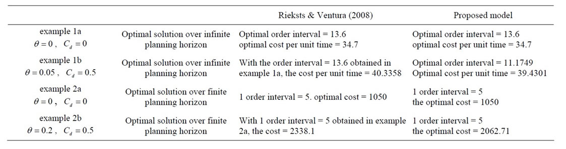
Table 1. Comparison between this study and Rieksts and Ventura (2008).
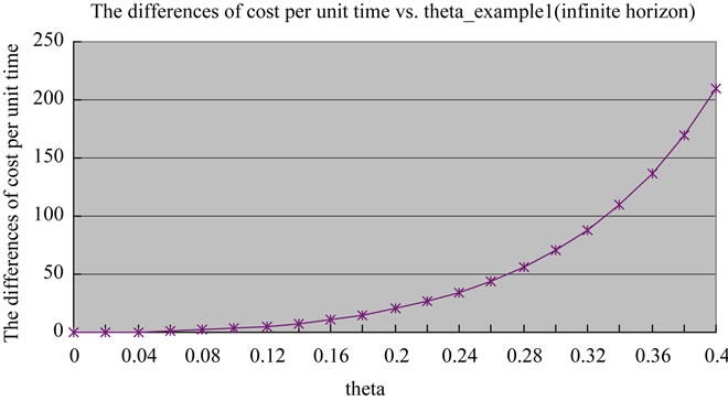
Figure 1. The differences of cost per unit time vs. the deterioration rate (in example 1a and 1b: infinite planning horizon case).

Figure 2. The differences of cost vs. the deterioration rate (in example 2a and 2b: finite planning horizon case).
of costs between the two models increase with the rising deterioration rate ( ). The results of the proposed model perform better compared to the inventory model proposed by Rieksts and Ventura [1] when deterioration rate (
 ) is large. It would be of interest to extend the model to situations where the retailer receives random demand before the customer’s real demand occurs.
REFERENCES
- B. Rieksts and J. Ventura, “Optimal Inventory Policies with Two Modes of Freight Transportation,” European Journal of Operational Research, Vol. 186, No. 2, 2008, pp. 576-585. doi:10.1016/j.ejor.2007.01.042
- S. K. Goyal and B. C. Giri, “Recent Trends in Modeling of Deteriorating Inventory,” European Journal of Operational Research, Vol. 134, No. 1, 2001, pp. 1-16. doi:10.1016/S0377-2217(00)00248-4
- R. Li, H. Lan and J. R. Mawhinney, “A Review on Deteriorating Inventory Study,” Journal of Service Science and Management, Vol. 3, No. 1, 2010, pp. 117-129. doi:10.4236/jssm.2010.31015
- B. Rieksts and J. Ventura, “Two-Stage Inventory Models with a Bi-Modal Transportation Cost,” Computers and Operations Research, Vol. 37, No. 1, 2010, pp. 20-31. doi:10.1016/j.cor.2009.02.026
- D. Aucamp, “Nonlinear Freight Costs in the EOQ Problem,” European Journal of Operational Research, Vol. 9, No. 1, 1982, pp. 61-63. doi:10.1016/0377-2217(82)90011-X
- S. Lippman, “Economic Order Quantities and Multiple Set-Up Costs,” Management Science, Vol. 18, No. 1, 1971, pp. 39-47. doi:10.1287/mnsc.18.1.39
- C. Y. Lee, “The Economic Order Quantity for Freight Discount Costs,” IIE Transactions, Vol. 18, No. 3, 1986, pp. 318-320. doi:10.1080/07408178608974710
- H. Hwang, D. Moon and S. Shinn, “An EOQ Model with Quantity Discounts for both Purchasing Price and Freight Cost,” Computers and Operations Research, Vol. 17, No. 1, 1990, pp. 73-78. doi:10.1016/0305-0548(90)90029-7
- R. Tersine, S. Barman and R. Toelle, “Composite lot Sizing with Quantity and Freight Discounts,” Computers and Industrial Engineering, Vol. 28, No. 1, 1995, pp. 107-122. doi:10.1016/0360-8352(94)00031-H
- W. Adelwahab and M. Sargious, “Freight Rate Structure and Optimal Shipment Size in Freight Transportation,” Logistics and Transportation Review, Vol. 26, No. 3, 1990, pp. 271-292.
- S. Swenseth and M. Godfrey, “Incorporating Transportation Costs into Inventory Replenishment Decisions,” International Journal of Production Economics, Vol. 77, No. 2, 2002, pp. 113-130. doi:10.1016/S0925-5273(01)00230-4
- L. Burns, R. Hall and D. Blumenfeld, “Distribution Strategies That Minimize Transportation and Inventory Costs,” Operations Research, Vol. 33, No. 3, 1985, pp. 469-490. doi:10.1287/opre.33.3.469
- P. Larson, “The Economic Transportation Quantity,” Transportation Journal, Vol. 28, No. 2, 1988, pp. 43-48.
- K.-J. Chung and C.-N. Lin, “Optimal Inventory Replenishment Models for Deteriorating Items Taking Account of Time Discounting,” Computers and Operations Research, Vol. 28, No. 1, 2001, pp. 67-83. doi:10.1016/S0305-0548(99)00087-8
- L. Benkherouf, A. Boumenir and L. Aggoun, “A Diffusion Inventory Model for Deteriorating Items,” Applied Mathematics and Computation, Vol. 138, No. 1, 2003, pp. 21-39. doi:10.1016/S0096-3003(02)00097-8
- K. J. Heng, J. Labban and R. L. Lim, “An Order-Level Lot Size Inventory Model for Deteriorating Items with Finite Replenishment Rate,” Computer and Industrial Engineering, Vol. 20, No. 2, 1991, pp. 187-197. doi:10.1016/0360-8352(91)90024-Z
- F. Raafat, P. M. Wolfe and H. K. Eldin, “An Inventory Model for Deteriorating Items,” Computers and Industrial Engineering, Vol. 20, No. 2, 1991, pp. 89-94. doi:10.1016/0360-8352(91)90043-6
- C. H. Goh, B. S. Greenberg and H. Matsuo, “Two-Stage Perishable Inventory Models,” Management Science, Vol. 39, No. 5, 1993, pp. 633-649. doi:10.1287/mnsc.39.5.633
- H. Yan and T. C. E. Cheng, “Optimal Production Stopping and Restarting Times for an EOQ Model with Deterioration Items,” Journal of the Operational Research Society, Vol. 49, No. 12, 1998, pp. 1288-1295.
- B. C. Giri, T. Chakrabarty and K. S. Chaudhuri, “A Note on a Lot Sizing Heuristic for Deteriorating Items with Time Varying Demands and Shortages,” Computers and Operations Research, Vol. 27, No. 6, 2000, pp. 495-505. doi:10.1016/S0305-0548(99)00013-1
- J.-T. Teng, H.-J. Chang, C.-Y. Dye and C.-H. Hung, “An Optimal Replenishment Policy for Deteriorating Items with Time-Varying Demand and Partial Backlogging,” Operations Research Letters, Vol. 30, No. 6, 2002, pp. 387-393. doi:10.1016/S0167-6377(02)00150-5
- K.-J. Chung, P. Chu and S.-P. Lan, “A Note on EOQ Models for Deteriorating Items under Stock Dependent Selling Rate,” European Journal of Operational Research, Vol. 124, No. 3, 2000, pp. 550-559. doi:10.1016/S0377-2217(99)00203-9
- B. C. Giri and K. S. Chaudhuri, “Deterministic Models of Perishable Inventory with Stock-Dependent Demand Rate and Nonlinear Holding Cost,” European Journal of Operational Research, Vol. 105, No. 3, 1998, pp. 467-474. doi:10.1016/S0377-2217(97)00086-6
- D. K. Bhattachaya, “Production, Manufacturing and Logistics on Multi-Item Inventory,” European Journal of Operational Research, Vol. 162, No. 3, 2005, pp. 786- 791.
- K.-S. Wu, L.-Y. Ouyang and C.-T. Yang, “An Optimal Replenishment Policy for Non-Instantaneous Deteriorating Items with Stock-Dependent Demand and Partial Backlogging,” International Journal of Production Economics, Vol. 101, No. 2, 2006, pp. 369-384. doi:10.1016/j.ijpe.2005.01.010
- H. M. Wee, “A Replenishment Policy for Items with a Price-Dependent Demand and a Varying Rate of Deterioration,” Production Planning and Control, Vol. 8, No. 5, 1997, pp. 494-499. doi:10.1080/095372897235073
- H.-M. Wee and S.-T. Law, “Economic Production Lot Size for Deteriorating Items Taking Account of the TimeValue of Money,” Computers and Operations Research, Vol. 26, No. 6, 1999, pp. 545-558. doi:10.1016/S0305-0548(98)00078-1
- P. M. Ghare and G. P. Schrader, “A Model for an Exponentially Decaying Inventory,” Journal of Industrial Engineering, Vol. 14, No. 5, 1963, pp. 238-243.
- Y. K. Shah and M. C. Jaiswal, “An Order-Level Inventory Model for a System with Constant Rate of Deterioration,” Opsearch, Vol. 14, 1977, pp. 174-184.
- G. Padmanabhana and P. Vratb, “EOQ Models for Perishable Items under Stock Dependent Selling Rate,” European Journal of Operational Research, Vol. 86, No. 2, 1995, pp. 281-292. doi:10.1016/0377-2217(94)00103-J
- A. K. Bhunia and M. Maiti, “An Inventory Model of Deteriorating Items with Lot-Size Dependent Replenishment Cost and a Linear Trend in Demand,” Applied Mathematical Modeling, Vol. 23, No. 4, 1999, pp. 301-308. doi:10.1016/S0307-904X(98)10089-6
- A. K. Bhunia and M. Maiti, “Deterministic Inventory Model for Deteriorating Items with Finite Rate of Replenishment Dependent on Inventory Level,” Computers and Operations Research, Vol. 25, No. 11, 1998, pp. 997- 1006. doi:10.1016/S0305-0548(97)00091-9
- P. L. Abad, “Optimal Price and Order Size for a Reseller under Partial Backordering,” Computers and Operations Research, Vol. 28, No. 1, 2001, pp. 53-65. doi:10.1016/S0305-0548(99)00086-6
- S. Mukhopadhyay, R. N. Mukherjee and K. S. Chaudhuri, “Joint Pricing and Ordering Policy for a Deteriorating Inventory,” Computers and Industrial Engineering, Vol. 47, No. 4, 2004, pp. 339-349. doi:10.1016/j.cie.2004.06.007
- N. K. Mahapatra, “Decision Process for Multi-Objective, Multi-Item Production-Inventory System via Interactive Fuzzy Satisficing Technique,” Computers and Mathematics with Applications, Vol. 49, No. 5, 2005, pp. 805- 821. doi:10.1016/j.camwa.2004.07.020
- L. Schwarz, “Economic Order Quantities for Products with Finite Demand Horizons,” AIIE Transactions, Vol. 4, No. 3, 1972, pp. 234-237. doi:10.1080/05695557208974855
Appendix A
Proof of Proposition 1: Rieksts and Ventura [1] presented proofs similar to proposition 1 and proposition 7-10. Proof is given by contradiction. Let  denote the inventory level at time t and
  denote the quantity ordered at time t. Suppose there is an optimal ordering policy that does not satisfy the zero-inventory ordering property at time
  that is the order time closest to time
  and
and . We consider another ordering policy at time (
 ). The holding cost of this adjusted policy is reduced by
 . This contradicting the optimality of ordering policy, therefore the optimal ordering policy over finite planning horizon will satisfy the zero inventory policy. The similar argument can extend to infinite planning horizon.
Appendix B
Proof of Proposition 2:
Let
 therefore
  is a increasing function and
 , i.e.,
Therefore . A similar argument also shows that
 .
.
Appendix C
Proof of Proposition 3: Redefine
 ,
,  and
and  . By the intermediate value theorem, there exist a
  such that
 . i.e.,
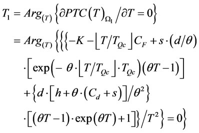
Redefine ,
,  and
and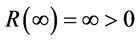 . By the intermediate value theoremthere exist a
  such that
 . i.e.,
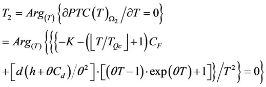
Therefore we can find  in
in  and
and  in
in  by setting
 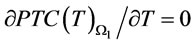 and
and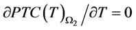 .
.
Appendix D
Proof of Proposition 4: We get
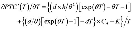
and
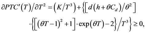
therefore  is a convex function. Redefine
 , we find
  and
and . By the intermediate value theorem, there exist a
  such that
 . Where

Therefore we can find  that is the optimal order interval that minimize
 .
.
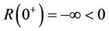
Appendix E
Proof of Proposition 5: The statement
 is equivalent to the statement
 .
.
Proof by contradiction.  is the optimal order interval that minimize
  (defined in proposition 4). Only the average holding and setup costs included in
  represent a convex function with a minimum in
 .
.
Suppose that the optimal order interval  of
of  is not on the interval
where
 .
.
We first consider . Since the average holding and setup costs represent a convex function with a minimum on the interval
 , the average holding cost and setup costs for
  are more than for
 . The average transportation cost at
 is at a minimum since full cargo loads are used. This implies that the average cost at
  is greater than the cost at
 . A similar argument also shows that the cost at
  is greater than the cost at
 . This contradicting the optimality of
 , therefore the optimal order interval
  of
of
 is in the range
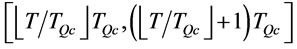
where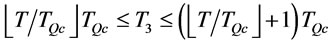 .
.
Appendix F
Proof of Proposition 7: Proof is given by contradiction. Suppose that there are  order times in the optimal ordering policy. This implies that there are at least two order intervals,
  and
and  such that
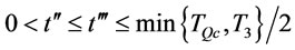 . Consider a ordering policy that is identical to the optimal ordering policy except that the order intervals
  and
and  are combined into a single order interval. Because the average holding and setup costs included in
  represent a convex function with a minimum in
  and
and 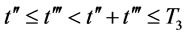 , the average holding and setup cost the adjusted policy is lower than the optimal ordering policy. Otherwise the average transportation cost is not increased in the adjusted policy since
  . Thus the total cost of the adjusted policy is less than the optimal ordering policy. This contradicting the optimality of ordering policy, therefore the optimal order times over finite planning horizon is at most
Appendix G
Proof of Proposition 8: Proof is given by contradiction. Suppose that the optimal ordering policy has at least two order intervals  and
and  such that
 . We consider another ordering policy that is analogous to the optimal ordering policy with two order intervals
  and
and . In the adjusted policy, the set up cost and transportation cost are kept unchanged, but the holding cost of the adjusted policy is reduced by
 . This contradicting the optimality of ordering policy, therefore
 .
.
Appendix H
Proof of Proposition 9: Proof is given by contradiction. Suppose that there exist an order interval
 in the optimal ordering policy. Let
  for arbitrarily j and m be the cardinality of the set
 . Because
  and
and  (proposition 8),
 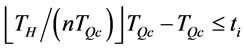 . In two cases1)
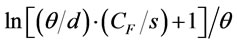
 and 2)
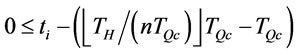
 considering another ordering policy that is analogous to the optimal ordering policy with two order intervals
  and
and . For case 1), let
  and
and
 . Because the average holding and setup costs in cost function is a convex function of t and
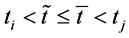 , then the holding cost and set up cost of the adjusted policy (order intervals
 ,
, ) is less than the policy (
 ). And transportation cost are kept unchanged since

and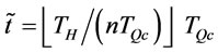 . Hence the total cost of the adjusted policy is less than the optimal ordering policy in case 1). For case 2), let
 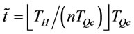 and
and
 ,
,
 m be the cardinality of the set
 . Because
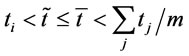 , then the holding cost and set up cost of the adjusted policy is reduced due to equality of order intervals. And transportation cost are kept unchanged since
Hence the total cost of the adjusted policy is less than the optimal ordering policy in case (2). This contradicts the optimality of ordering policy. Similar argument is also hold in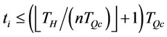 . Therefore, if
  is an optimal order interval with n order times,
 .
.
Appendix I
Proof of Proposition 10: Proposition 10 is equivalent to the statement as follows:  and
and  are any two order intervals in an optimal ordering policy. If 1):
  and
and  fall in
simultaneously or 2)  and
and  fall in
simultaneously, then .
.
Proof is given by contradiction. Suppose that two order intervals  and
and  in the optimal ordering policy is such that
 where
where 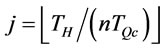 (by proposition 9). We consider another ordering policy that is analogous to the optimal ordering policy but two order intervals
  and
and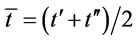 .
.
implies that
 .
.
In the adjusted policy, the set up cost and transportation cost are kept unchanged, but the holding cost of the adjusted policy is reduced due to equality of order intervals (see Schwarz [36]). This contradicting the optimality of ordering policy, and similar proof is also proved in
 .
.
Therefore if  and
and  fall in

simultaneously or (2)  and
and  fall in
simultaneously, then .
.
Appendix J
Proof of Proposition 11: Given n and , minimizing the objective function
  in (32) with respect to
 . We get
Therefore  is a convex function. Redefine
 ,
,  and
and
 . By the intermediate value theorem, there exist a
  such that
 . Where
Therefore we can find  that minimizes
  .
.