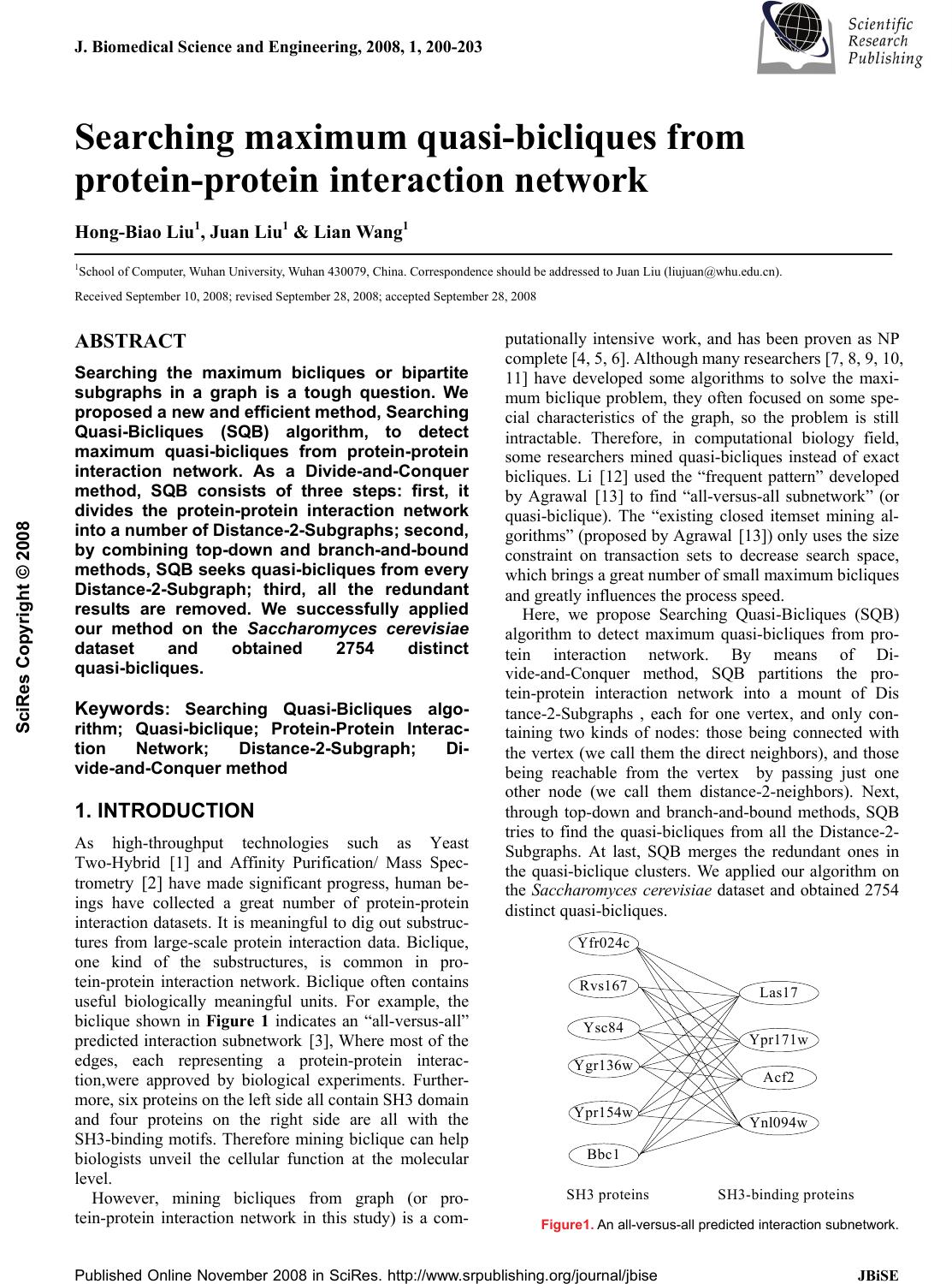J. Biomedical Science and Engineering, 2008, 1, 200-203
Published Online November 2008 in SciRes. http://www.srpublishing.org/journal/jbise JBiSE
Searching maximum quasi-bicliques from
protein-protein interaction network
Hong-Biao Liu1, Juan Liu1 & Lian Wang1
1School of Computer, Wuhan University, Wuhan 430079, China. Correspondence should be addressed to Juan Liu ([e-mail]).
Received September 10, 2008; revised September 28, 2008; accepted September 28, 2008
ABSTRACT
Searching the maximum bicliques or bipartite
subgraphs in a graph is a tough question. We
proposed a new and efficient method, Searching
Quasi-Bicliques (SQB) algorithm, to detect
maximum quasi-bicliques from protein-protein
interaction network. As a Divide-and-Conquer
method, SQB consists of three steps: first, it
divides the protein-protein interaction network
into a number of Distance-2-Subgraphs; second,
by combining top-down and branch-and-bound
methods, SQB seeks quasi-bicliques from every
Distance-2-Subgraph; third, all the redundant
results are removed. We successfully applied
our method on the Saccharomyces cerevisiae
dataset and obtained 2754 distinct
quasi-bicliques.
Keywords: Searching Quasi-Bicliques algo-
rithm; Quasi-biclique; Protein-Protein Interac-
tion Network; Distance-2-Subgraph; Di-
vide-and-Conquer method
1. INTRODUCTION
As high-throughput technologies such as Yeast
Two-Hybrid [1] and Affinity Purification/ Mass Spec-
trometry [2] have made significant progress, human be-
ings have collected a great number of protein-protein
interaction datasets. It is meaningful to dig out substruc-
tures from large-scale protein interaction data. Biclique,
one kind of the substructures, is common in pro-
tein-protein interaction network. Biclique often contains
useful biologically meaningful units. For example, the
biclique shown in Figure 1 indicates an “all-versus-all”
predicted interaction subnetwork [3], Where most of the
edges, each representing a protein-protein interac-
tion,were approved by biological experiments. Further-
more, six proteins on the left side all contain SH3 domain
and four proteins on the right side are all with the
SH3-binding motifs. Therefore mining biclique can help
biologists unveil the cellular function at the molecular
level.
However, mining bicliques from graph (or pro-
tein-protein interaction network in this study) is a com-
putationally intensive work, and has been proven as NP
complete [4, 5, 6]. Although many researchers [7, 8, 9, 10,
11] have developed some algorithms to solve the maxi-
mum biclique problem, they often focused on some spe-
cial characteristics of the graph, so the problem is still
intractable. Therefore, in computational biology field,
some researchers mined quasi-bicliques instead of exact
bicliques. Li [12] used the “frequent pattern” developed
by Agrawal [13] to find “all-versus-all subnetwork” (or
quasi-biclique). The “existing closed itemset mining al-
gorithms” (proposed by Agrawal [13]) only uses the size
constraint on transaction sets to decrease search space,
which brings a great number of small maximum bicliques
and greatly influences the process speed.
Here, we propose Searching Quasi-Bicliques (SQB)
algorithm to detect maximum quasi-bicliques from pro-
tein interaction network. By means of Di-
vide-and-Conquer method, SQB partitions the pro-
tein-protein interaction network into a mount of Dis
tance-2-Subgraphs , each for one vertex, and only con-
taining two kinds of nodes: those being connected with
the vertex (we call them the direct neighbors), and those
being reachable from the vertex by passing just one
other node (we call them distance-2-neighbors). Next,
through top-down and branch-and-bound methods, SQB
tries to find the quasi-bicliques from all the Distance-2-
Subgraphs. At last, SQB merges the redundant ones in
the quasi-biclique clusters. We applied our algorithm on
the Saccharomyces cerevisiae dataset and obtained 2754
distinct quasi-bicliques.
Yfr024c
Rvs167
Ysc84
Ypr154w
Bbc1
Las17
Ypr171w
Acf2
Ynl094w
Ygr136w
SH3 proteinsSH3-binding proteins
Figure1. An all-versus-all predicted interaction subnetwork.
SciRes Copyright © 2008

H. B. Liu / J. Biomedical Science and Engineering 1 (2008) 200-203 201
SciRes Copyright © 2008 JBiSE
The organization of this paper is as follows. Section 2
states the maximum Quasi-biclique problem. Section 3
describes the SQB algorithm for finding the maximum
quasi bicliques. Section 4 reports the results of the ap-
plication of SQB algorithm on in a real proteomic data.
The paper ends with conclusions and the future work.
2. MAXIMUM QUASI-BICLIQUE
PROBLEM
We use a simple graph like [14] to describe a pro-
tein-protein interaction network. A vertex represents a
kind of protein and an edge means there is an interaction
between two kinds of proteins. Quasi-biclique is a graph
G= (V, E), in which V can be divided into two non empty
sets {V1, U1} and every vertex in V1 directly links to
nearly every vertex in U1. The question of finding
maximum quasi-biclique in a graph G= (V, E) can be
formalized as following function.
,)),((
)),((max
nmEVGf
EVGf
=
subject to VUVVUV
VmnUmVn
⊂⊂=∩
≤+==
1,1,11
|,||,1||,1|
φ
where |V| denotes cardinality of the vertex set of the input
graph, n and m should be greater than 1 and lower than
|V|-2. A quasi-biclique is measured by the value of nm
which actually is the number of interacting edges between
two sets. In the following, we denote a quasi-bicluque as
QB (V1, U1).
3. SQB ALGORITHM
The main method of SQB is Divide-and-Conquer, which
includes three parts. The first one is to seek every ver-
tex’s Distance-2-Subgraph from a graph. The second one
is to find every vertex’s quasi-biclique from its Dis-
tance-2-Subgraph. The third one is to merge solutions:
after finding every vertex’s quasi-bicliques, SQB puts all
the quasi-bicliques together, removes the similar ones,
prunes the smaller ones, and obtains the quasi-bicliques
of the whole graph. The three parts of SQB are detailed
in the following.
3.1. Finding Distance-2-Subgraph
As some graph, especially the biological protein-protein
interaction network, is very large, the process on the graph
will need a very large memory space so it is not feasible in
common applications. But it is obvious that the distance
between any two vertexes in a quasi-biclique is not greater
than 2. So if we want to find a quasi-biclique which in-
cludes a specific vertex, we only need to consider the
vertex and its related neighbors. The related neighbors are
vertexes which are less than 3 in distance to the specific
vertex. The induced subgraph, which consists of the ver-
tex and its related neighbors, is denoted as Dis-
tance-2-Subgraph. The edge status between any two ver-
texes in an induced subgraph is the same as that in the
original graph. SQB needs to find every vertex’s Dis-
tance-2-Subgraph in order to obtain its maximum
quasi-biclique.
3.2. Detecting Maximum Quasi-bicliques
After finding every vertex’s Distance-2-Subgraph, SQB
begins to find the quasi-biclique. This process, detecting
quasi-bicliques, is the essential part of SQB. SQB uses the
size (nm) to measure a quasi-biclique and it is crucial to
know the specific value of n and m of a maximum
quasi-biclique. As n and m are in a limited range, SQB
tests the values of n and m from the upper limit to the
lower one. If a graph has a quasi-biclique QB(|V|=n,
|U|=m), the vertexes in the graph with degree lower than n
and m should not be in the QB, so SQB removes these
smaller vertexes during the process. Furthermore, if the
test value of n and m are greater, SQB can remove more
vertexes and increase the speed of the process.
Before explaining our program, we introduce how to
split a graph. We use a complex data structure CD to store
the V1 set, U1 set and the induced subgraph G of V1 set
and U1 set. The program splits the graph at the V1 set, and
U1 set in turn. The program chooses the vertex in V1 or
U1 with largest degree and labels it so that next time, the
program avoids splitting at the same vertex again. For
example, if the program chooses v15 as the candidate
vertex, it then produces four sets V150, V151, U150, and
U151. The first set V150 includes v15 and vertexes in V1
which has a distance of 2 to vertex v15. The second set
V151 consists of elements in V1 except v15. The third set
U150 contains vertexes in U1 which is the direct neighbor
of vertex v15. The fourth set U151 is the same as U1. Next,
the program produces induced graph G150 which con-
tains vertexes V150 and U150, then puts V150, U150,
G150 into data structure CD150(V150, U150, G150). In
the same way, it gets another data structure CD151(V151,
U151, G151).
The algorithm of detecting quasi-bicliques is listed in
the end of this subsection. The algorithm consists of a
FOR loop that begins from 20 to 2. (20 is an experimental
value which should be increased with the growing of
nodes of the input graph). At first SQB uses the
sub-function Search_k_Quasi_Bicliques(G, k) to test
whether the graph contains quasi-bicliques in which the
|V|>20 and |U|>20. If the sub-function finds it’s true, the
FOR loop terminates, otherwise the FOR loop decreases
the test value by one and continues to test, until the
sub-function finds quasi-bicliques or the test value lower
than 2.
The sub-function func Search_k_Quasi_Bicliques(G, k)
is the key component of SQB. At first, the input graph G’s
vertex set is divided into two parts, V1 and U1. Next, V1
and U1, and G are put into complex data structure CD(V1,
U1, G). CD is put into a buffer BUFFER. Next, the pro-
gram go into a WHILE loop. This loop’s terminate con-
dition is that the buffer is empty. During the loop, first, the
program removes one element from BUFFER and puts it
into CD0(V01, U01, G0), then deletes vertex in V01 with

202 H. B. Liu / J. Biomedical Science and Engineering 1 (2008) 200-203
SciRes Copyright © 2008 JBiSE
degree lower than k and deletes vertex in U01 with degree
lower than k. Next, the program judges whether CD0(V01,
U01, G0) is a quasi-biclique. If the CD0 is a
quasi-biclique and the size is greater than the current
maximum value, the program outputs CD0 and puts the
current maximum value as CD0’s size. If it is not a
quasi-biclique and its size greater than current maximum
value, the program splits the CD0 into two units (CD01,
CD02) and puts them into the BUFFER. Otherwise, the
program discards the left smaller ones.
Part of SQB Algorithm
Input. Graph G(V, E)
Output. The maximum quasi-bicliques in G(V, E)
func Search_Maximum_Quasi_Bicliques() =
for tt from 20 to 2 step-1 do
OUT= Search_k_Quasi_Bicliques(G, tt)
If OUT is not empty
Output OUT and Stop the program
end for
end func Search_Maximum_Quasi_Bicliques()
func Search_k_Quasi_Bicliques(G, k)=
Divide vertex set V into two sets, V1 and U1
Put V1, V2, G into Complex Data Structure CD(V1, U1,
G)
Put CD into BufferBUFFER
While(BUFFER is not empty)
Remove first element in BUFFER to CD0(V01, U01,
G0)
Delete vertex in V01 with degree lower than k
Delete vertex in U01 with degree lower than k
If CD0(V01, U01, G0) is Quasi_Bicliques
then output CD0
Else if CD0(V01, U01, G0) is not empty
then Split CD0 into CD01, CD02 at one unlabeled
vertex
put CD01, CD02 into BUFFER
end while
end func Search_k_Quasi_Bicliques()
3.3. Pruning Redundant Quasi-bicliques
Through the above steps, SQB obtains every vertex’s
quasi-bicliques. As some vertexes might have similar
quasi-bicliques, SQB needs to remove redundant ones and
obtains the overall distinct quasi-bicliques of the whole
graph. SQB deletes one between any two quasi-bicliques
QB1(V1, U1) and QB2(V2, U2) if they meet the follow-
ing rules:
If V2))(U1U2)((V1||2))(U1 )21((⊆∩⊆⊆
∩
⊆UVV is true,
then delete QB1.
If ))12()12((||))1(U2 )12((VUUVUVV ⊆∩⊆⊆
∩
⊆ is true,
then delete QB2.
The first rule means that if V1 is V2’s subset and U1 is
U2’s subset, or if V1 is U2’s subset and U1 is V2’s subset,
then QB1 is a part of QB2, QB1 can be deleted. The
second rule is opposite to the first one. Otherwise, if two
quasi-bicliques match neither of the above two rules, SQB
keeps both of them.
After the pruning operation, SQB obtains the distinct
quasi-bicliques of the whole graph and the biggest one is
the optimum one of the whole graph.
4. APPLICATION OF SQB
The experiment was done on our web server which con-
sisted of two Pentium 2 PCs with 4.8 GHZ CPU and 2G
RAM. The Saccharomyces cerevisiae dataset Y78, de-
rived from [15], consists of 78,390 protein-protein inter-
actions, including 5321 proteins. During our experiments,
we removed vertexes with degree 1 because they could
not produce a biclique. The input graph of our program is
with node number 4546. At first, we produced 4546 dis-
tinct Distance-2-Subgraphs according to every vertex’s
neighbors and their neighbors. The maximum subgraph is
with 3164 nodes and the average value is 746.1. So the
questions are very tough.
About eighty percent of the vertexes have a process
time less than 20 seconds and half of them are processed
within 1 second. The average time is about 13.4 seconds.
Giving the large input graphs, the performance is very
remarkable.
During our experiments we predicted 5616 quasi-bi-
cliques which include empty or redundant ones. A small
number of vertexes have more than one maximum
quasi-bicliques, so the number of quasi-bicliques is
greater than 4546, the number of Distance-2-Subgraphs.
Table 1. The Maximum Quasi-Bicliques (YPL212C).
|V|=26 YBL038W YBR251W YBR283C YDL136W YDL191W YEL050C YGL103W YGL123W YGR034W
YGR220C YIL018W YIL021W YJL063C YLR075W YLR344W YLR378C YMR260C YNL178W YNL284C
YNR037C YOL040C YOL127W YOR063W YPL131W YPL183W-A YPR110C
|U|=62
YBL087C YBL091C YBR031W YBR048W YBR146W YCR031C YDL061C YDL083C YDL140C
YDL202W YDR012W YDR025W YDR101C YDR116C YDR226W YDR237W YDR418W YDR450W
YEL054C YER117W YER170W YFL001W YGL063W YGL068W YGL135W YGL147C YGR085C
YHR147C YIL133C YJL177W YJL190C YJL191W YKL009W YKL024C YKL170W YKL180W YLR244C
YLR340W YLR367W YLR388W YML010W YML025C YML026C YMR143W YMR158W YMR188C
YNL067W YNL069C YNL081C YNL177C YNL185C YNL306W YOR116C YOR150W YOR151C
YOR207C YOR341W YPL212C YPL220W YPR010C YPR102C YPR166C

H. B. Liu / J. Biomedical Science and Engineering 1 (2008) 200-203 203
SciRes Copyright © 2008 JBiSE
0
200
400
600
800
1000
1200
1400
1600
1800
01000 20003000 4000 5000
Vertex sorted by Size
Quasi-biclique Size
Figure 2. The size of maximum quasi-biclique of every vertex
The size of quasi-biclique is measured by the prod
uct of n=|V| and m=|U|. Figure 2 shows the size of
every vertex’s maximum quasi-biclique. The average
value is 115.8. The largest one is with size 1612=26*62
which includes protein YPL212C and is listed in Table 1.
Every vertex in the protein set V touches every one in the
set U. During our experiments, we thought the
quasi-biclique with size lower than 4*4 is easy to occur
by random and should be discarded. At last we obtained
2754 distinct maximum quasi-bicliques which are avail-
able on our website http://biod.whu.edu.cn/pub/QuasiBi-
clique.txt.
5. CONCLUSION
In this study, we developed Searching Quasi-Bicliques
(SQB) algorithm to detect maximum quasi-biclique from
a large scale protein-protein interaction network. SQB
uses the Divide-and-Conquer method to process data.
Combination of Top-down method and the
branch-and-bound method greatly reduces the search
space. We successfully applied it to the analysis of Yeast
proteomic data and obtained many quasi-bicliques, which
might provide meaningful clues to potential biological
users.
Although we obtained some quasi-bicliques, they
might not be global optimum ones because the results are
influenced by the choice of start splitting vertex. In addi-
tion, we might integrate more biological features, such as
the proteins’ functional category, to analyze the mecha-
nism of the quasi-biclique in the cell.
ACKNOWLEDGEMENTS
This work is partially supported by the National Nature Science
Foundation of China under grant 3010.
REFERENCES
[1] S. Fields and R. Sternglanz. (1994) The two-hybrid system: an
assay for protein-protein interactions, Trends Genet, 10(8),
286-292.
[2] A.Bauer and B. Kuster. (2003) Affinity purification-mass spec-
trometry. Powerful tools for the characterization of protein com-
plexes, Eur J Biochem, 270(4), 570-578.
[3] A.H.Tong, B.Drees, et al.( 2002) A combined experimental and
computational strategy to define protein interaction networks for
peptide recognition modules, Science, 295(5553), 321-324.
[4] M.R.Garey, D.S. Johnson, et al.( 1976) Some simplified
NP-complete graph problems, Theoretical Computer Science, 1(3):
237-267.
[5] R.M. Karp. (1972) Reducibility among combinatorial problems,
Complexity of Computer Computations, 43, 85-103.
[6] S.Even and Y. Shiloach. (1975) NP-completeness of several ar-
rangement problems, Dept. Computer Science, Technion, Haifa,
Israel, Tech. Rep, 43.
[7] J.A. Bondy and S.C. Locke (1986) Largest bipartite subgraphs in
triangle-free graphs with maximum degree three, Journal of graph
theory, 10(4), 477-504.
[8] M. Grotschel and W.R. Pulleyblank (1981) Weakly bipartite
graphs and the max-cut problem, Operations Research Letters,
1(23-27), 482.
[9] F. Barahona. (1983) On some weakly bipartite graphs, Operations
Research Letters, 5, 239242.
[10] J.J. Hopfield and D.W. Tank (1985) "Neural" computation of
decisions in optimization problems, Biological Cybernetics, 52(3),
141-152.
[11] J.J. Hopfield. (1984) Neurons with Graded Response Have Collec-
tive Computational Properties like Those of Two-State Neurons,
Proceedings of the National Academy of Sciences of the United
States of America, 81(10), 3088-3092.
[12] H. Li, J. Li, et al.( 2006) Discovering motif pairs at interaction
sites from protein sequences on a proteome-wide scale, Bioinfor-
matics, 22(8), 989-996.
[13] R. Agrawal and R. Srikant (1994) Fast Algorithms for Mining
Association Rules in Large Databases, Proceedings of the 20th
International Conference on Very Large Data Bases, 487-499.
[14] N. Pržulj, (2004) Graph theory approaches to protein interaction
data analysis, in Knowledge Discovery in High-Throughput Bio-
logical Domains, Interpharm/CRC.
[15] C. von Mering, R. Krause, et al. (2002) Comparative assessment
of large-scale data sets of protein-protein interactions, Nature,
417(6887), 399-403.