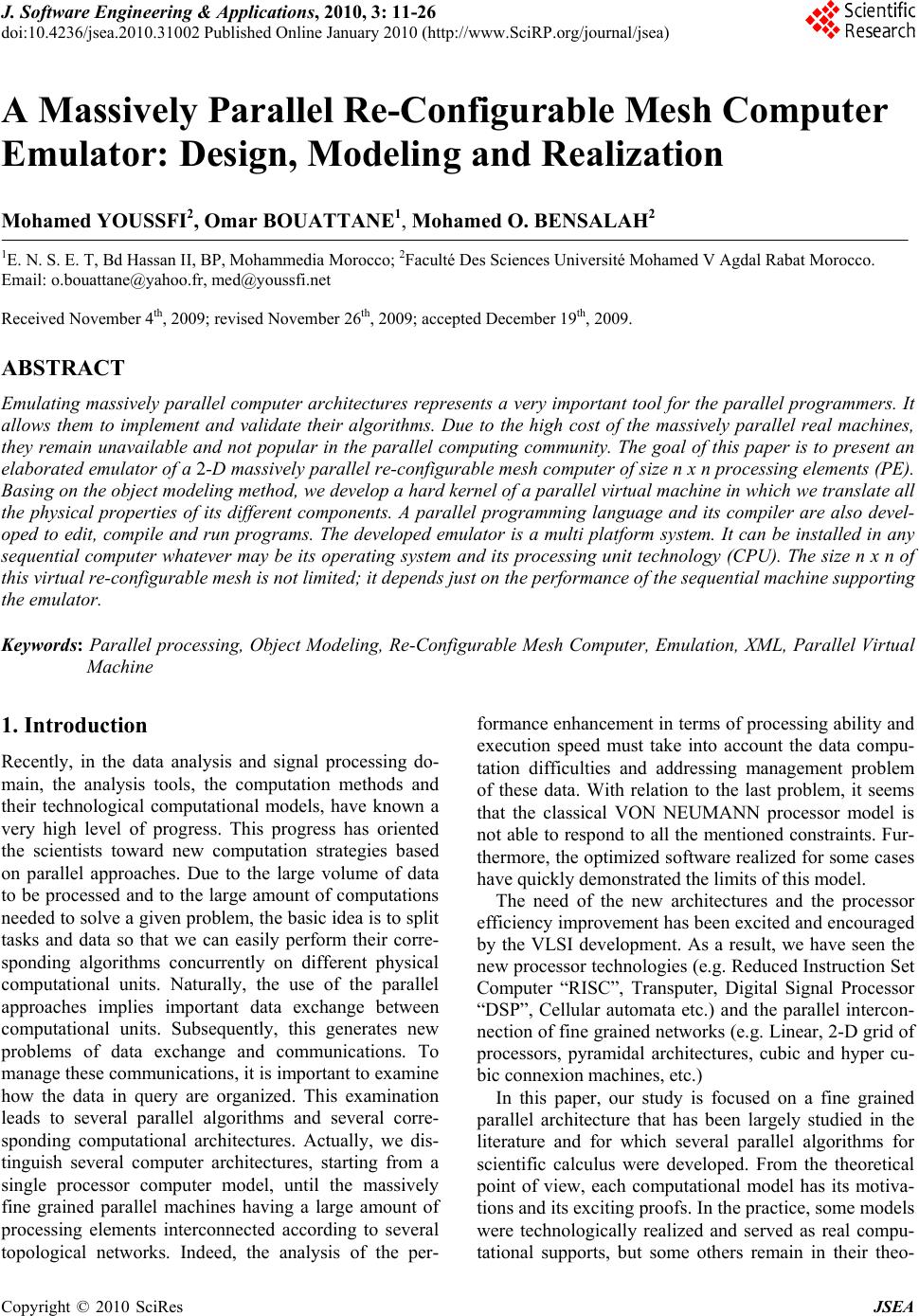J. Software Engineering & Applications, 2010, 3: 11-26
doi:10.4236/jsea.2010.31002 Published Online January 2010 (http://www.SciRP.org/journal/jsea)
11
A Massively Parallel Re-Configurable Mesh Computer
Emulator: Design, Modeling and Realization
Mohamed YOUSSFI2, Omar BOUATTANE1, Mohamed O. BENSALAH2
1E. N. S. E. T, Bd Hassan II, BP, Mohammedia Morocco; 2Faculté Des Sciences Université Mohamed V Agdal Rabat Morocco.
Received November 4th, 2009; revised November 26th, 2009; accepted December 19th, 2009.
ABSTRACT
Emulating massively parallel computer architectures represents a very important tool for the parallel programmers. It
allows them to implement and validate their algorithms. Due to the high cost of the massively parallel real machines,
they remain unavailable and not popular in the parallel computing community. The goal of this paper is to present an
elaborated emulator of a 2-D massively parallel re-configurable mesh computer of size n x n processing elements (PE).
Basing on the object modeling method, we develop a hard kernel of a parallel virtual machine in which we translate all
the physical properties of its different components. A parallel programming language and its compiler are also devel-
oped to edit, compile and run programs. The developed emulator is a multi platform system. It can be installed in any
sequential computer whatever may be its operating system and its processing unit technology (CPU). The size n x n of
this virtual re-configurable mesh is not limited; it depends just on the performance of the sequential machine supporting
the emulator.
Keywords: Parallel processing, Object Modeling, Re-Configurable Mesh Computer, Emulation, XML, Parallel Virtual
Machine
1. Introduction
Recently, in the data analysis and signal processing do-
main, the analysis tools, the computation methods and
their technological computational models, have known a
very high level of progress. This progress has oriented
the scientists toward new computation strategies based
on parallel approaches. Due to the large volume of data
to be processed and to the large amount of computations
needed to solve a given problem, the basic idea is to split
tasks and data so that we can easily perform their corre-
sponding algorithms concurrently on different physical
computational units. Naturally, the use of the parallel
approaches implies important data exchange between
computational units. Subsequently, this generates new
problems of data exchange and communications. To
manage these communications, it is important to examine
how the data in query are organized. This examination
leads to several parallel algorithms and several corre-
sponding computational architectures. Actually, we dis-
tinguish several computer architectures, starting from a
single processor computer model, until the massively
fine grained parallel machines having a large amount of
processing elements interconnected according to several
topological networks. Indeed, the analysis of the per-
formance enhancement in terms of processing ability and
execution speed must take into account the data compu-
tation difficulties and addressing management problem
of these data. With relation to the last problem, it seems
that the classical VON NEUMANN processor model is
not able to respond to all the mentioned constraints. Fur-
thermore, the optimized software realized for some cases
have quickly demonstrated the limits of this model.
The need of the new architectures and the processor
efficiency improvement has been excited and encouraged
by the VLSI development. As a result, we have seen the
new processor technologies (e.g. Reduced Instruction Set
Computer “RISC”, Transputer, Digital Signal Processor
“DSP”, Cellular automata etc.) and the parallel intercon-
nection of fine grained networks (e.g. Linear, 2-D grid of
processors, pyramidal architectures, cubic and hyper cu-
bic connexion machines, etc.)
In this paper, our study is focused on a fine grained
parallel architecture that has been largely studied in the
literature and for which several parallel algorithms for
scientific calculus were developed. From the theoretical
point of view, each computational model has its motiva-
tions and its exciting proofs. In the practice, some models
were technologically realized and served as real compu-
tational supports, but some others remain in their theo-

A Massively Parallel Re-Configurable Mesh Computer Emulator: Design, Modeling and Realization 12
retical proposition state. They are not realized because of
their technological complexities and to their very high
production cost. The computational model that is con-
cerned in our work has known a very large technological
progress. At first, it was viewed as a simple grid of cel-
lular automata, after some technological enhancement,
the cellular automaton became a fine grained processing
element and the resulted grid became the mesh connected
computer MCC [1]. Using some additional communica-
tion Buses, the MCC became the mesh with multiple
broadcast [2] and polymorphic torus [3]. Finally, we
speak about the reconfigurable mesh computer (RMC)
that integrates a reconfiguration network at each proc-
essing element [4,5].
From the algorithmic point of view, several authors
were developed new parallel algorithms for data proc-
essing and scientific calculus. These algorithms were
assigned to be implemented in the architectures men-
tioned above. Also, they are established using parallel
approaches in order to reduce their complexities in term
of execution times.
In order to facilitate for each parallel programmer the
task of validation and program tests (even if he has not a
real parallel machine that supports his algorithms), the
emulating solutions were proposed in the literature to
elaborate some virtual systems to perform the algorithms.
The emulated systems may be specific as in [21,22] or of
general behaviors as in [19,20].
In this context, we present in this paper a virtual tool
to emulate an RMC, in which we can easily implement
parallel SIMD algorithms. It is a virtual RMC platform
of size (n x m) processing elements (PE), where n is the
number of rows in the matrix an m is the number of
columns. Without loss of generality, we consider n = m
and we speak about a squared matrix of n² PE’s.
This emulator allows the scientists to overflow the
problem of real RMC availability. (i.e. at this time the
RMC machine is not yet popular due to its high cost).
Using this emulator, we propose an extended virtual
RMC model, which translates all the functionalities of a
real machine. This model can be easily extended to per-
form other advanced functionalities required by the mul-
tiplicity of the algorithmic techniques. In order to reach
this virtual machine result, we started by the object mod-
eling of all the components of the RMC such as the n x n
grid, its processing element PE, its connexion buses and
so. To describe in more details the different steps of this
emulator realization, we organize this paper as follows:
Section II presents the real RMC model and the essential
properties of its components. The object modeling of the
RMC and some related details are given in section III.
The next section, presents some parallel programs and
their implementation on our virtual machine to illustrate
the use of some established parallel instructions. Notice
that, to avoid the upload of this paper, the complete set of
instructions established for our platform is not presented
in more details. We present just some examples of testing
programs that involve some scientific computations such
as basic matrix computation, data processing and image
processing. Finally, the last section gives some conclud-
ing remarks and some exploiting perspectives of our vir-
tual machine.
2. Parallel Computational Model
2.1 Presentation
The parallel architectures have known a large develop-
ment these recent years. They are presented in numerous
topological shapes, such as, linear, planar, pyramidal,
cubic and hyper cubic networks. This large number of
architectures requires an adequate classification taking
into account several criteria. Among these criteria, we
distinguish for example, the size of the machine, its
autonomy of addressing and connexion, data type used
etc. This classification allows the programmer to choose
an appropriate computational model to perform the pro-
grams. Several proposed classifications were described in
the literature; the diversity of the architectural solutions
makes difficult the establishment of a general taxonomy.
The well known classification is based on multiplicity of
the instruction and data flows. It proposed four types of
data machines, they are: the Single Instruction Single
Data (S.I.S.D), single Instruction Multiple Data (S.I.
M.D), multiple Instruction Single Data (M.I.S.D) and
multiple Instruction Multiple Data (M.I.M.D) machines.
Throughout this classification, the concerned model in
this work is the Re-configurable Mesh Computer. It is
the 2-D planar grid or matrix of n x n processing ele-
ments (PE). It is an S.I.M.D structure where in the word
model the PE’s use data buses of width at most log2 n
bits. Also, in this model, the PE’s has the autonomy of
operation, addressing and connexion.
2.2 Topology and Structure
A Re-configurable Mesh Computer (RMC) of size n x n,
is a parallel machine having n2 Processing elements
(PE’s) arranged on a 2-D matrix as shown in Figure 1. It
is a “Single Instruction Multiple Data (SIMD)” structure,
Figure 1. Re-configurable mesh computer model of size 8 x 8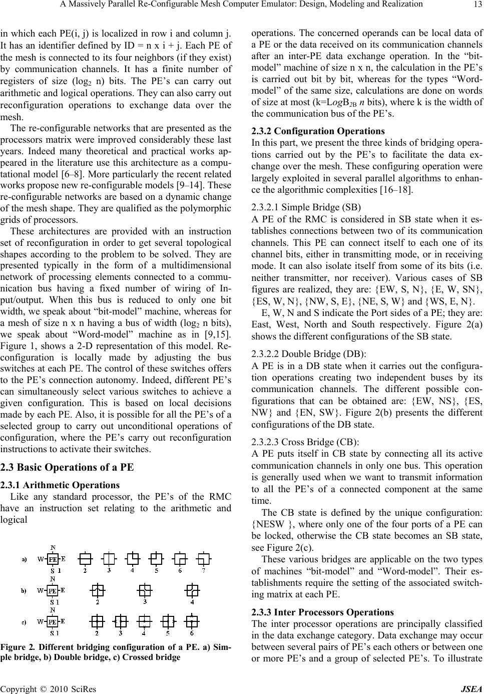

A Massively Parallel Re-Configurable Mesh Computer Emulator: Design, Modeling and Realization13
in which each PE(i, j) is localized in row i and column j.
It has an identifier defined by ID = n x i + j. Each PE of
the mesh is connected to its four neighbors (if they exist)
by communication channels. It has a finite number of
registers of size (log2 n) bits. The PE’s can carry out
arithmetic and logical operations. They can also carry out
reconfiguration operations to exchange data over the
mesh.
The re-configurable networks that are presented as the
processors matrix were improved considerably these last
years. Indeed many theoretical and practical works ap-
peared in the literature use this architecture as a compu-
tational model [6–8]. More particularly the recent related
works propose new re-configurable models [9–14]. These
re-configurable networks are based on a dynamic change
of the mesh shape. They are qualified as the polymorphic
grids of processors.
These architectures are provided with an instruction
set of reconfiguration in order to get several topological
shapes according to the problem to be solved. They are
presented typically in the form of a multidimensional
network of processing elements connected to a commu-
nication bus having a fixed number of wiring of In-
put/output. When this bus is reduced to only one bit
width, we speak about “bit-model” machine, whereas for
a mesh of size n x n having a bus of width (log2 n bits),
we speak about “Word-model” machine as in [9,15].
Figure 1, shows a 2-D representation of this model. Re-
configuration is locally made by adjusting the bus
switches at each PE. The control of these switches offers
to the PE’s connection autonomy. Indeed, different PE’s
can simultaneously select various switches to achieve a
given configuration. This is based on local decisions
made by each PE. Also, it is possible for all the PE’s of a
selected group to carry out unconditional operations of
configuration, where the PE’s carry out reconfiguration
instructions to activate their switches.
2.3 Basic Operations of a PE
2.3.1 Arithmetic Operations
Like any standard processor, the PE’s of the RMC
have an instruction set relating to the arithmetic and
logical
Figure 2. Different bridging configuration of a PE. a) Sim-
ple bridge, b) Double bridge, c) Crossed bridge
operations. The concerned operands can be local data of
a PE or the data received on its communication channels
after an inter-PE data exchange operation. In the “bit-
model” machine of size n x n, the calculation in the PE’s
is carried out bit by bit, whereas for the types “Word-
model” of the same size, calculations are done on words
of size at most (k=LogB2B n bits), where k is the width of
the communication bus of the PE’s.
2.3.2 Configuration Operations
In this part, we present the three kinds of bridging opera-
tions carried out by the PE’s to facilitate the data ex-
change over the mesh. These configuring operation were
largely exploited in several parallel algorithms to enhan-
ce the algorithmic complexities [16–18].
2.3.2.1 Simple Bridge (SB)
A PE of the RMC is considered in SB state when it es-
tablishes connections between two of its communication
channels. This PE can connect itself to each one of its
channel bits, either in transmitting mode, or in receiving
mode. It can also isolate itself from some of its bits (i.e.
neither transmitter, nor receiver). Various cases of SB
figures are realized, they are: EW, S, N, E, W, SN,
ES, W, N, NW, S, E, NE, S, Wand WS, E, N.
E, W, N and S indicate the Port sides of a PE; they are:
East, West, North and South respectively. Figure 2(a)
shows the different configurations of the SB state.
2.3.2.2 Double Bridge (DB):
A PE is in a DB state when it carries out the configura-
tion operations creating two independent buses by its
communication channels. The different possible con-
figurations that can be obtained are: EW, NS, ES,
NW and , SW. Figure 2(b) presents the different
configurations of the DB state.
2.3.2.3 Cross Bridge (CB):
A PE puts itself in CB state by connecting all its active
communication channels in only one bus. This operation
is generally used when we want to transmit information
to all the PE’s of a connected component at the same
time.
The CB state is defined by the unique configuration:
NESW , where only one of the four ports of a PE can
be locked, otherwise the CB state becomes an SB state,
see Figure 2(c).
These various bridges are applicable on the two types
of machines “bit-model” and “Word-model”. Their es-
tablishments require the setting of the associated switch-
ing matrix at each PE.
2.3.3 Inter Processors Operations
The inter processor operations are principally classified
in the data exchange category. Data exchange may occur
between several pairs of PE’s each others or between one
or more PE’s and a group of selected PE’s. To illustrate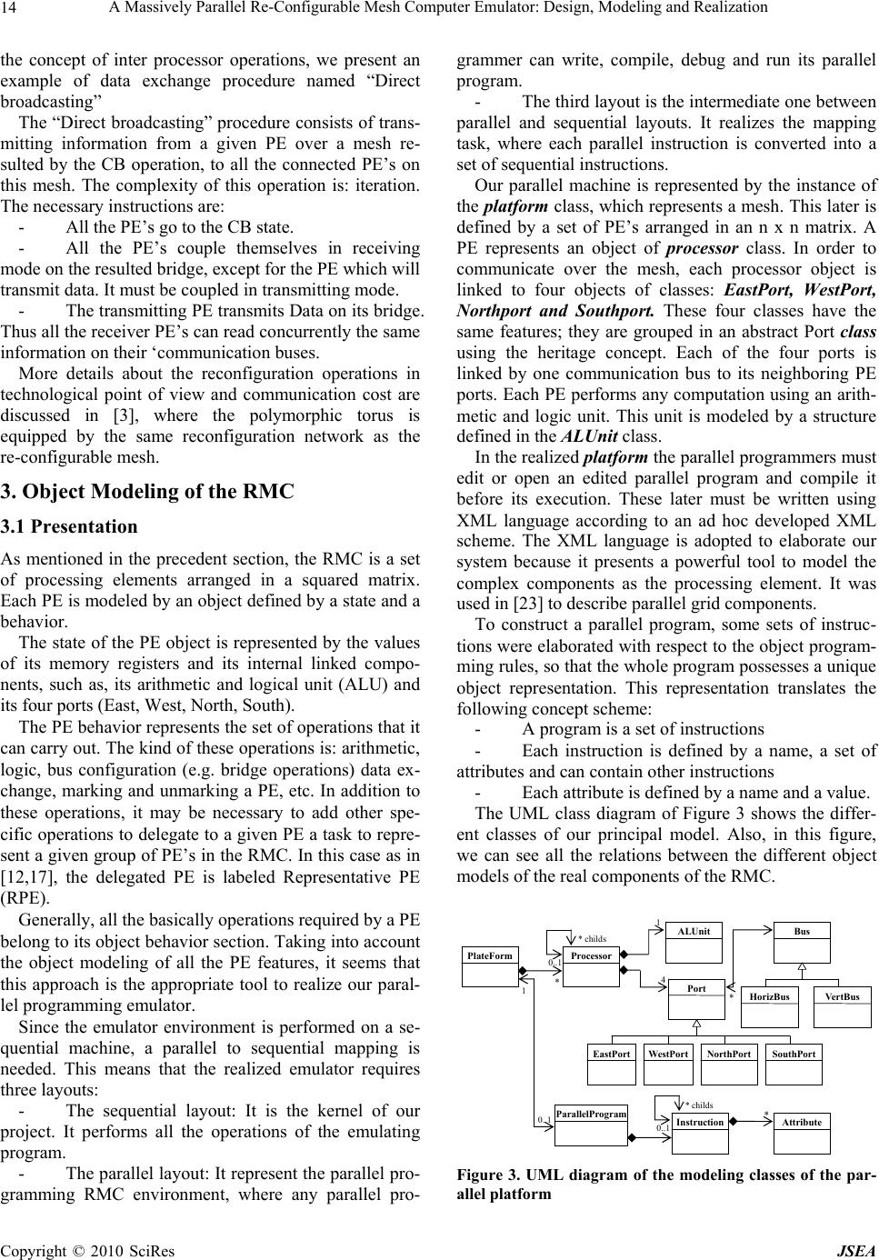

A Massively Parallel Re-Configurable Mesh Computer Emulator: Design, Modeling and Realization 14
the concept of inter processor operations, we present an
example of data exchange procedure named “Direct
broadcasting”
The “Direct broadcasting” procedure consists of trans-
mitting information from a given PE over a mesh re-
sulted by the CB operation, to all the connected PE’s on
this mesh. The complexity of this operation is: iteration.
The necessary instructions are:
- All the PE’s go to the CB state.
- All the PE’s couple themselves in receiving
mode on the resulted bridge, except for the PE which will
transmit data. It must be coupled in transmitting mode.
- The transmitting PE transmits Data on its bridge.
Thus all the receiver PE’s can read concurrently the same
information on their ‘communication buses.
More details about the reconfiguration operations in
technological point of view and communication cost are
discussed in [3], where the polymorphic torus is
equipped by the same reconfiguration network as the
re-configurable mesh.
3. Object Modeling of the RMC
3.1 Presentation
As mentioned in the precedent section, the RMC is a set
of processing elements arranged in a squared matrix.
Each PE is modeled by an object defined by a state and a
behavior.
The state of the PE object is represented by the values
of its memory registers and its internal linked compo-
nents, such as, its arithmetic and logical unit (ALU) and
its four ports (East, West, North, South).
The PE behavior represents the set of operations that it
can carry out. The kind of these operations is: arithmetic,
logic, bus configuration (e.g. bridge operations) data ex-
change, marking and unmarking a PE, etc. In addition to
these operations, it may be necessary to add other spe-
cific operations to delegate to a given PE a task to repre-
sent a given group of PE’s in the RMC. In this case as in
[12,17], the delegated PE is labeled Representative PE
(RPE).
Generally, all the basically operations required by a PE
belong to its object behavior section. Taking into account
the object modeling of all the PE features, it seems that
this approach is the appropriate tool to realize our paral-
lel programming emulator.
Since the emulator environment is performed on a se-
quential machine, a parallel to sequential mapping is
needed. This means that the realized emulator requires
three layouts:
- The sequential layout: It is the kernel of our
project. It performs all the operations of the emulating
program.
- The parallel layout: It represent the parallel pro-
gramming RMC environment, where any parallel pro-
grammer can write, compile, debug and run its parallel
program.
- The third layout is the intermediate one between
parallel and sequential layouts. It realizes the mapping
task, where each parallel instruction is converted into a
set of sequential instructions.
Our parallel machine is represented by the instance of
the platform class, which represents a mesh. This later is
defined by a set of PE’s arranged in an n x n matrix. A
PE represents an object of processor class. In order to
communicate over the mesh, each processor object is
linked to four objects of classes: EastPort, WestPort,
Northport and Southport. These four classes have the
same features; they are grouped in an abstract Port class
using the heritage concept. Each of the four ports is
linked by one communication bus to its neighboring PE
ports. Each PE performs any computation using an arith-
metic and logic unit. This unit is modeled by a structure
defined in the ALUnit class.
In the realized platform the parallel programmers must
edit or open an edited parallel program and compile it
before its execution. These later must be written using
XML language according to an ad hoc developed XML
scheme. The XML language is adopted to elaborate our
system because it presents a powerful tool to model the
complex components as the processing element. It was
used in [23] to describe parallel grid components.
To construct a parallel program, some sets of instruc-
tions were elaborated with respect to the object program-
ming rules, so that the whole program possesses a unique
object representation. This representation translates the
following concept scheme:
- A program is a set of instructions
- Each instruction is defined by a name, a set of
attributes and can contain other instructions
- Each attribute is defined by a name and a value.
The UML class diagram of Figure 3 shows the differ-
ent classes of our principal model. Also, in this figure,
we can see all the relations between the different object
models of the real components of the RMC.
PlateForm Processor
ALUnit
Port
EastPort WestPort NorthPort SouthPort
Bus
HorizBus Ver tB us
ParallelProgram Instruction Attribute
0..1
* childs
4
*
1
0..1
0..1
* childs
*
*
1
Figure 3. UML diagram of the modeling classes of the par-
allel platform

A Massively Parallel Re-Configurable Mesh Computer Emulator: Design, Modeling and Realization15
Data Re
g
isters
idReg
Flag register
0 1 2 3 ......15
bridge
A
L
U
P
O
R
T
P
O
R
T
PORT
PORT
BUS
BUS
BUS
iReg
jReg
Reg[2]
Reg[1]
Reg[0]
Reg[n]
BUS
Figure 4. Representation of the components of a processing
element model
3.2 Description of the RMC Model Classes
3.2.1 Processor Class
In this part, we have translated all the physical compo-
nents of a PE as in Figure 4, and its functionalities to the
processor model. The defined processor class must take
into account all the elementary functions and the set of
the elementary physical parts of the PE. Thus, each PE is
defined by its state, its behavior and must have an iden-
tity.
3.2.1.1 Processing Element State
The state model of a PE describes all its physical com-
ponents. They are:
Identifier registers:
When a created PE is inserted in the mesh model, its
instance variables iReg and jReg which represent its lo-
cation coordinates in the n x n matrix are set. The identi-
fier register of this PE idReg, will take the value com-
puter in the row major order by: idReg = n*iReg+ jReg.
Internal registers:
For any given computation problem, each PE must use
some internal registers to save data and the results of any
related processing. To do so, we define in the PE model
an array of internal data registers named “reg [..]”. In
this model, we have defined arbitrarily an array of 16
data registers. This array may be extended dynamically
to any other size according to the problem in query.
Flags:
As any standard processor, we introduce in the PE
model a special flag register, where each of its flag bits
will indicate the PE state related to any performed in-
struction. This register is arbitrarily defined by an array
of 16 bits, but it can be extended to any large size ac-
cording to any additional useful instruction.
Communication Ports:
In the real RMC machine, all the PE’s can exchange
data via their communication ports, between each others
what ever their locations in the matrix. In order to ac-
complish this task in the modeled machine, the commu-
nication ports of a PE are represented by objects linked
to the PE using the reference indicators stored in the de-
fined variables: eastport, westport, northPort and south-
Port.
ALUnit:
To perform advanced logical and arithmetical opera-
tions, each PE uses its ALUnit. This later is modeled by
an object of the class ALUnit and having a reference
stored in the variable named ALUnit.
Other components:
Notice that the RMC machine emulator is an open sys-
tem. It can be dynamically and easily extended in terms
of register memories, communication bus width, and
special functions according to the problem in query. For
example: In the image processing domain and for some
specific applications, some hierarchical strategies are
often used to enhance the complexity of the correspond-
ing algorithms. (e.g. q-tree based algorithms, component
contour based algorithms, labeling etc.). In such cases, of
special advanced programming applications, some algo-
rithms require special additional variables or registers.
The programmer has the ability to extend easily its com-
putational model.
To illustrate the proposition of this part, we consider
an example where a PE can be representative of a group
of other PE’s. To do so, we define in the processor class
a collection of objects of type processor. In this collec-
tion we save the represented PE identifiers. Furthermore,
a given PE can easily know its representative PE using
the representative PE variable which contains the identi-
fier of its representative PE. This representative property
was largely used in the literature as in [12,17].
3.2.1.2 Processing Element Behavior
The behavior of the PE is implemented by methods in-
side the processor class. These methods are classified in
three categories.
Basically operations: The basically operations that
can carry out a PE are the same as in any standard proc-
essor. Thus in this part we have implemented the meth-
ods to model the arithmetic operations (addition, subtrac-
tion, multiplication, division, etc.). Also we have imple-
mented two operations to model some complex arithme-
tic and logic expressions. They are named: executeArit-
hmeticExpression() and executeLogicExpression(). These
expressions may respect the format imposed by C++ and
java programming language. To do so, we have created a
logic and arithmetic expression compiler using a com-
plex process. This process is not presented in this paper
because it is not the main idea discussed in this work.
Several other methods have been defined in this class
to offer to the programmer a large library of useful meth-
ods and operations.
Data exchange operations: The previous operations
can be viewed as a category belonging to the set of in-
structions of any sequential programming language. Par-

A Massively Parallel Re-Configurable Mesh Computer Emulator: Design, Modeling and Realization 16
allel programming is characterized by other types of in-
structions. In fact, as mentioned above, the Peps of the
RMC must collaborate between each others by exchang-
ing data via their communication buses. Among the im-
plemented methods of this category, we distinguish:
 sendValue (double v): This method allows the
PE to send a data value v to its neighboring PE’s accord-
ing to its bridge configuration state.
 receiveData (double data, char port, byte regR):
Allows the PE to receive a data value on its port speci-
fied by the parameter port and to store the received data
in its register regR.
 sendAndReceiveData (char portS, byte regS,
char portR, byte regR): allows the PE to send the data
value of its register regS on the port specified by the pa-
rameter portS, and receive data on the port specified by
the parameter portR, the PE stores the received data in its
register regR.
 receiveAndSendWithOperation (ProcessPort po-
rt, String op): This method is used to receive data, exe-
cute some operations on this data and send the result to
other PE’s according to their bridge states.
Configuration operations: In the parallel program-
ming domain and particularly in the SIMD computational
models, the processing element can play several roles
depending on its configurations. In the processor class,
we have defined a set of methods to change and to know
the actual configuration of the PE. During the execution
phase of a given parallel program, it is necessary to point
at each stage of this phase, the group of active PE’s. For
these reasons, we define the methods select() and un-
select() to select or unselect the Peps that are susceptible
to execute or not the instructions. Among the selected
PE’s, it is possible to assign for some specific instruc-
tions the concerned PE’s using other methods to mark or
unmark them. Thus, we define other methods, mark()
and unmark() to distribute a Boolean label to each se-
lected PE. This label can be integrated in the program as
a test variable.
To determine the configuration state of a PE at any
given stage, some other appropriate operations are intro-
duced.
The methods associated to the configuration opera-
tions depend usually on the content of the flags register.
Figure 5 summarizes the significance and the usefulness
of each bit of this register where:
3.2.2 ALUnit Class
In a given parallel program, the PE’s must be able to
perform the arithmetical and logical expressions defined
by any mathematical expression using all the possibilities
of a programming language like java. During the compi-
lation procedure, the mathematical expressions must be
compiled and stored in temporary files to be used during
their execution. The static methods defined in the
ALUnit class named, createArithmeticExpression() and
createLogicExpression() are used to compile the arith-
metic and logic expression. To run the previous compiled
expression, we can use the following two methods:
 getLogicExpression(int index,ArrayList params):
returns the result of the logical expression of the instruc-
tion numbered by the index parameter. If this expression
is included in an iterative loop, the iteration values will
be stored in the array param s.
 executeArithmericOperation(int index, Array-
List params): executes the arithmetic expression of the
instruction numbered by index. If this expression is in-
cluded in an iterative loop, the iteration values will be
stored in the array param s.
3.2.3 Port Class
As mentioned above, each PE possesses four communi-
cation ports. Each port is associated to a communication
bus. In our model, we define four types of ports: East,
West, North and South. All these four ports have the
same characteristics; they are grouped in an abstracted
Port class.
A port is an object having a state defined by a label
(N,E,W,S) and a reference ” process” to the processor
object to which it belongs.
Bit number 0 1 2 3 4 5 6 7 8 9 10 11 12 13 14 15
State (x =0 or 1) x X x x x x x x X
 Bit 0 : indicates if the PE is marked or not.
 Bit 1 : indicates if the PE is selected or not.
 Bit 2 : indicates if the state of the PE is changed or not.
 Bit 3 : indicates if the PE has loaded data or not.
 Bit 4 : indicates if the PE has a representative PE or not.
 Bit 12 : indicates if the last executed logical operation is valid or not.
 Bit 13 : indicates if the PE has received data or not.
 Bit 14 : indicates if the PE is a representative or not.
 Bit 15 : shows if the parity flag of the PE is true or false.
 Bits 5 to 11 are not used, they are available to define other states in the PE.
Figure 5. The content of the flags register of a modeled PE

A Massively Parallel Re-Configurable Mesh Computer Emulator: Design, Modeling and Realization17
PlateForm
ParalleleProgram
fileName: String
compile(): void
run
()
: voi
d
1
1
Instruction
name: String
execute(): void
1..*
Attribute
name: String
value : String
0..*
1..1 1..1
0..*
0..1
Figure 6. The UML class diagram of a program
A port can be locked by its PE using a Boolean in-
stance variable locked. Since each port is associated to a
communication bus, the reference to this bus must be
stored in this class. Finally, each port must have one con-
figuration variable to specify how the data can be trans-
ferred from the port to its communication bus.
Example: If we consider an 8 bits communication bus,
the defaults configuration of a port is defined by the or-
der «01234567». This means that the bit i (i=0 to 7) of
the port is linked to the bit i of the bus. In this case the
data sent over the port is transmitted without any trans-
formation. While in the configuration «70123456» the bit
0 of the port is connected to bit 1 of the bus and the bit i
(i=1 to 6) is linked to bit i+1 of the bus. The bit 7 of the
port is linked to bit 0 of the bus. This means that the
transmitted data is left rotated over the bus. This kind of
commutation operations on ports are often used in
several parallel programs [9].
3.3 Parallel Program Object Modeling
A parallel program loaded in the plate- form is composed
by a set of instruction. Each instruction is defined by zero
or several attributes. An instruction contains the child
instructions and belongs to a father instruction. The class
sheet of Figure 6 shows the class diagram of this model.
3.3.1 Parallel Program Class
A parallel program is defined by the source file name of
this program. This source file is created by the program-
mer with the extension “.par” and must respect the XML
norm. The program is defined by the variables: firstIn-
struction, lastInstruction and currentInstruction that rep-
resent the first, the last and the current instruction of the
program (respectively). Some other instance variables are
defined like: endCompilation to indicate if the compila-
tion of the program is finished. iterationLevel to store the
current iteration level in the loop cases.
To run an edited program, we begin by the method
compile(). The compiling procedure acts as follows:
- read the program source file
- load it in the memory as a tree of instructions
- The first instruction is stored in the firstInstruc-
tion variable.
- The last instruction is stored in the lastInstruc-
tion variable.
- Execute the program starting from the first in-
struction.
3.3.2 Instruction Class
To edit a parallel program in this emulator, we have cre-
ated a parallel programming language using our specific
XML scheme. Each instruction of this language is de-
fined by several attributes and can contain other instruc-
tions. Each attribute is an object of the attribute class
which is self defined by its name and its value. In the
program, each instruction is viewed as a tree structure. It
is delimited by a beginning and ending tags. Between
these tags, we can find other child instructions having the
same structure. Between the tags of the child instruction,
we can find other child instructions having the same
structure etc. For this reason, an instruction is defined by
a dynamic table named childs, to store the references to
the other child instruction objects. Furthermore, an in-
struction can know its father thanks to the variable “par-
ent” which contains its parent reference. Finally, there
are other interesting variables used during the execution
of the instruction, they are defined in this class, such as,
opened and executed variables that indicate if the instruc-
tion is opened or executed.
Example:
<for-eachPE test="reg[0]>0">
<mark/>
<doOperation expression="reg[0]=(reg[1]+reg[2])/2"/>
</for-eachPE>
In this example scheme, we show the structure of the
parallel instruction «fo r-ea chPE ». It is defined by an
attribute «test» having the value «reg[0]>0». This in-
struction contains two instructions: The first is «mark»
which is without attribute, the second is the «do Opera-
tion» instruction having an attribute of name «expres-
sion» and value «reg[0]=(reg[1]+reg[2])/2».
This simple program example selects in the matrix of
processors all the PE’s having a positive value in their
registers reg[0]. The selected PE’s are marked (labeled).

A Massively Parallel Re-Configurable Mesh Computer Emulator: Design, Modeling and Realization 18
Then, all these marked PE’s perform the arithmetic op-
eration on their own data registers, reg[1] and reg[2] .
Finally the result of each PE is stored in its reg[0] regis-
ter. Figure 7 presents the object structure of the precedent
example after its compilation.
3.4 Platform Class
The modeled parallel machine is represented by an object
of the Platform class. In this paper, we are interested in
the implementation of the mesh as a matrix of n x n PE’s.
But, we can easily extend the model to other architec-
tures such as: Pipe line, Pyramidal machine etc. The
RMC model is characterized by the rows and cols vari-
ables that define the size of the matrix. The matrix crea-
tion is made by a matrix process[rows][cols] of object
processor (PE). The size of the resulted virtual mesh is
dynamically configurable and is not limited. It depends
only on the available memory space in the used sequen-
tial machine supporting the emulator.
In addition to the PE’s matrix, the platform is associ-
ated to an object representing the loaded and compiled
parallel program. Some additional Boolean variables are
used to complete the Platform state such as:
- Debug , to indicate whether the step by step
execution mode is activated
- DrawMode, to indicate the type of the graphic
context used in the displaying data zone.
- Compile, to indicate whether the loaded pro-
gram is compiled or not.
- Etc.
The most important part of this emulator is imple-
mented in the behavior part of the class platform. After
loading a program using the method loadProgramme(),
we can run the compile() met h od to construct the instruc-
tions tree of the parallelProgram Object. For each of
these constructed parallel instructions trees, we realize
the parallel to sequential mapping task. Subsequently,
this task translates each parallel instruction into a set of
iterative sequential instructions.
In order to exploit the platform class to run a given
parallel program, we classify all its defined methods into
the following four categories:
3.4.1 Loading data on the mesh
In this category, we use some methods to load data in the
mesh which is the matrix of PE’s before any processing
procedure. As example, we distinguish the following:
- loadImage (): loads data image of any format
(bmp, jpg, png, gif) in the matrix of PE’s.
- loadMatrix(): loads a data matrix from a text file
to the matrix of PE’s.
- loadRandom Matrix(): computes and loads a
random data matrix in the mesh.
Notice that, all the used data types in any program-
ming language are supported by the modeled PE’s (e.g.
Byte, int, long, float, double etc.).
3.4.2 Configuration of the Mesh
In the SIMD parallel programming domain, it is neces-
sary to select the PE’s that are susceptible to perform
some given instructions. For this reasons, we have de-
fined the selection methods basing on different criteria.
We will discuss some ones in the instruction set part.
After any selection, the method executeConfig(String
conf) asks the selected PE’s to execute a configuration
operation.
3.4.3 Execution of the Program
After loading data and configuring the mesh, we can
perform the other instructions of the parallel program
related to the loaded data. The principal method used in
this part is ExecuteInstruction (Instruction ins). This
category of instructions concerns all the data processing
and scientific calculus operations.
:ParallelProgram
fileName = "prog1.par"
:Instruction
name = "for-eachPE"
:Attribute
name = "test"
value = "reg[0]>0"
:Instruction
name = "mark"
:Instruction
name = "doOperation"
:Attribute
name = "expression"
value="reg[0]=(reg[1]+reg[2])/2"
Figure 7. Object representation of an instruction

A Massively Parallel Re-Configurable Mesh Computer Emulator: Design, Modeling and Realization19
3.4.4 Displaying Results
During the program execution, we can insert some
methods to display the results using several numerical
formats. For example, we can use the text format to ob-
serve the contents of different registers of the PE’s or to
display any data results in text format. A graphical con-
text is also available in our platform to display other re-
sults in graphical mode such as curves and images.
3.5 Instruction Sets
In order to construct our programming language, we have
developed an XML scheme which defines the parallel
instruction sets to edit parallel programs.
A program must begin by the tag <prog> and ends by
</prog> tag. Between the two tags we can edit the in-
structions.
Each instruction begins by the tag indicating the in-
struction name and ends by the tag indicating the end of
the instruction. An instruction can be defined by several
attributes, it can encapsulate other instructions.
As for the real RMC, the emulating platform has three
categories of instruction sets. They are presented as fol-
lows:
3.5.1 Instructions for PE Configuration
In the SIMD architectures, the parallel programming is
based on a fundamental principle, where it is necessary
to select, mark and bridge the PE’s concerned by the in-
struction execution. The configuration instruction set is
expressed by the following actions:
Selecting: This action is expressed by the instruction:
<for-eachPE cols= "valCols" rows= "valRows"
test= "expression_logic" direction="">
… ( Operations to be executed )
</for-eachPE>
The attributes “cols” and “rows” define the concerned
columns and rows. When several columns and rows are
concerned, they are separated by commas.
The attribute direction is defined by a string to indi-
cate the direction of the selected group of PE’s starting
from the PE of coordinates indicated in “rows” and
“cols” attributes. The possible direction attributes are:
 «RE» or «RW»: to define the direction East or
West along a Row.
 «CN»or «CS»: to define the direction North or
South along a Column.
 «DNE» or «DNW»: for the direction North-Est
or North-West along a diagonal.
 «DSE» or «DSW»: for the direction South-Est
or South-West along a diagonal.
The attribute test is used to select a set of PE’s satis-
fying the condition defined by a logical expression.
For example, in the expression (test="reg[1]>10") ,
the selected PE’s are those having in their reg[1] the
values greater than 10.
Marking: This action uses the following instructions:
<mark type="true| false" />: to mark a PE if its at-
tribute type is true and unmark it, if this attribute is false.
<mark />: to mark a PE without condition.
<unMark />: to Unmark a PE without condition.
Bridging: As mentioned in the physical description of
the RMC, a PE can be configured in three kinds of
bridges: simple, double or crossed bridge. These bridging
states are implemented by the following instruction:
<bridge type= "SB-WE|SB-NS | SB-WN | SB-WS |
SB-NE | SB-SE | DB-WN-SE | DB-NE-SW |DB-NS-WE
| CB-WNE | CB-NES | CB-ESW | CB-SWN | CB-WNES
| NB"/>.
This instruction named bridge is used by a PE by de-
fining its kind in the attribute type.
The attribute type is formulated by:
- Defining the kind by: SB = Simple Bridge, DB=
Double Bridge and CB= Crossed Bridge.
- Defining the direction of the bridge E,W,N and
S for East, West, North and South (respectively)
The SB configurations are: {SB-NS, SB-WE, SB-WN,
SB-WS, SB-NE, SB-SE, SB-WS}.
At any mentioned configuration the data is bypassing
bi-directionally the PE over its bridges.
The DB configurations are: {DB-WN-SE, DB-NE-
SW, DB-NS-WE}.
In this case, two communication bridges are con-
structed by a PE. So, two data can simultaneously bypass
bi-directionally the PE.
The CB configurations are: {CB-WNE, CB-NES, CB-
ESW, CB-SWN, CB-WNES}.
In this case, the only one obtained communication
channel links at least three ports of the PE.
Notice that, to return back to the no bridge state from
any bridge configuration, we use the instruction bridge
with an attribute type {NB} to specify No Bridge.
3.5.2 Arithmetic / Logic Instructions and Control
Structures
In the modeled parallel programming language, the
arithmetic and logic instructions are expressed using the
format defined bellow. In addition to the reconfiguration
operations, each PE of the RMC can carry out a set of
arithmetic/logic instructions and control structures. These
instructions are formatted as defined in the following
examples:
- Arithmetic / logic instructions
<inc reg="numReg"/>: means: reg [numReg]
= reg [numReg]+1;
<dec reg="numReg"/>: means: reg [num-
Reg] = reg [numReg]-1;

A Massively Parallel Re-Configurable Mesh Computer Emulator: Design, Modeling and Realization 20
<add reg="numReg" value= "val"/>: means :
reg [numReg] = reg [numReg]+Value;
<sub reg="numReg" value= "val"/>: means :
reg [numReg] = reg [numReg]-Value;
<mult reg="numReg" value= "val"/>: means :
reg [numReg] = reg [numReg]*Value;
<div reg="numReg" value= "val"/>: means :
reg [numReg] = reg [numReg]/Value;
<doOperation expression= "arithmetic_expre-
ssion" />: This instruction executes the arithmetic ex-
pression specified by the expression attribute. We have
developped a compiler to execute all the possible arith-
metical expressions according to the same syntaxes of
the C and Java language.
- Control structures
The control structures defined for our platform are the
same as the well known for any language. The following
examples give the presentation of some structures.
<if test= "logic_ expression"> … instructions …
</if>
<for from= "begin_val" to= "end_val">… instruc-
tions ...</for>
<while test= "logic_expression">… instruction-
s …</while>
3.5.3 Data Exchange Instructions
The third instruction set developed for this emulator
concerns the specific instructions to exchange data be-
tween the PE’s of the RMC. This set allows the pro-
grammer to manipulate some new concepts introduced in
the parallel SIMD algorithms. These instructions use the
four Port objects of each PE to send, receive and broad-
cast data over the mesh. Among the defined instructions
we have:
<sendAndReceiveData portS="W|E|N|S" regS=""
portR="W|E|N|S" regR=""/>
This instruction allows the PE to send it Data from the
specified register regS to the port specified by port S
and to receive data from protR and save it in the register
regR.
<receiveAndTransmitData portS="W|E|N|S" regR
=" " data=" " />
This instruction indicates to the PE to receive data
specified by data attribute and store it in register regR
then send it from the port specified by protS.
3.6 Macro Commands and Parallel Functions
As any programming language, the macro commands
and functions are generated and inserted in specific li-
braries to facilitate their use in some advanced proce-
dures. In the same strategy, we have defined some paral-
lel macro commands and some functions to represent
some parallel pre-processing procedures which can be
inserted easily in any parallel program. The generated
library is subject to more extensions and developments.
In this section, we present some examples of Macro
commands and parallel functions to illustrate their use-
fulness as the pre-processing procedures.
Macro commands:
 <defineRepresentativePE-forEachRow />
This macro command is used to determine a represen-
tative PE of a group of marked PE’s for each row of the
mesh. This command it based on the Minimum value
search procedure at each row of the mesh. The output of
this command is the minimal identifier value (idReg)
found in at each group of marked PE’s in each row of the
mesh.
 <defineRepresentativePE-ForEachCol />
It is the same procedure used as in the precedent
macro command. But the Minimum value search proce-
dure is applied on columns instead of rows.
 <initialiseRepresentivePE />
This macro command is used to reset all the represen-
tative PE’s. In this case there is no representative of any
group of PE’s in the mesh. This means that each PE is
self representative.
 <doDistributeParityIndex from="W|E|N|S" />
This macro is used to distribute a special index named
“parity index”, alternatively to the marked PE’s a group.
It is an important macro command used as a pre-proc-
essing for some high level algorithms. This macro corre-
sponds to a procedure based on bridge and reconfigura-
tion operations where each marked PE receives on its
specified port a Boolean label “0” or “1”, and then it in-
verts it before sending it to its neighboring marked PE
according to the bridge state in which it is set.
Functions:
 isSelected( ): indicates if the PE is selected or
not. It uses the bit 1 of the flags register.
 isChanged( ): indicates if the state of the PE is
changed or not. This method is very useful in some
graphic refreshment procedures. It uses the bit 2 of the
flags register.
 isTestValide( ): indicates if the last executed
logical operation is valid or not.
 getParity( ): shows if the parity flag of the PE is
true or false. It uses the bit 15 of the flags register.
 isRepresentative( ): indicates if the PE is a
representative or not. It uses the bit 14 of the flags regis-
ter.
 hasReceivedData( ): indicates if the PE has re-
ceived data or not. It uses the bit 13 of the flags register.
 isMarked( ): indicates if the PE is marked or
not. It uses the bit 0 of the flags register.
 hasLoadedData( ): indicates if the PE has

A Massively Parallel Re-Configurable Mesh Computer Emulator: Design, Modeling and Realization 21
loaded data or not. It uses the bit 3 of the flags register.
 hasFinished( ): returns true value if all the
PE’s are in stand by mode. This function is called in the
stopping test of some iterative loops.
 hasRepresentant( ):indicates if the PE has a
representative PE or not.
 REGRep[numReg]: indicates the value of the
numReg register of its representative.
4. Applications
In this section, we present some parallel algorithm ex-
amples where some properties of the RMC are used to
examine how they are expressed using some instructions
of the instruction sets defined above.
Program 1: Example1.par
<prog>
<for-eachPE cols="0,2,4" rows="*">
<mark type="true"/>
<loadRandomIntValue minValue="10" max-
Value="255"/>
<if test="reg[0]>=100">
<bridge type="SB-NS"/>
</if>
</for-eachPE>
</prog>
The result if this program is described as follows:
- It selects all the PE’s of the column 0, 2 and 4.
Then all the selected PE’s are marked “true”.
- Each one of these marked PE’s must compute
and save in its memory register reg[0], a random data
having a value between minValue="10" and max-
Value="255".
All the selected PE’s having a data value greater than
or equal to 100 must configure themselves in Simple
Bridge of direction (North–South) NS.
Figure 8 shows the states of all the PE’s of the RMC
matrix after the program execution. The marked PE’s are
represented by the hashed squares. The NS bridge is rep-
resented by vertical lines linking its North and South
ports of the PE is SB state and its neighbors.
Program 2: Example2.par
This example shows the point to point mean computa-
tion of two data matrices.
<prog>
<loadMatrix file="matrix1.txt" reg="0"/>
<loadMatrix file="matrix2.txt" reg="1"/>
<for-eachPE cols="*" rows="*">
<mark type="true"/>
<doOperation expres-
sion="reg[2]=(reg[0]+reg[1])"/>
</for-eachPE>
</prog>
We consider two data matrices saved in the data files
«matrix1.txt» and «matrix2.txt» respectively. The results
of the different stages of this program example are:
- The first matrix is mapped to the RMC of the
same size as this matrix, one element per PE. At each PE
the element is stored in its Reg [0] register.
- The second matrix is mapped to the RMC of the
same size as this matrix, one element per PE. At each PE
the element is stored in its Reg [1] register.
- All the PE’s of the RMC are selected and marked.
Reg[0]
Marked PE
UnMarked PE
PE in State
SB
North South
1234
0
1
2
3
4
0
43
0
0
0
0
0
23
0
0
0
0
0
32
0
0
12
0
0
0
0
0
134
0
0
0
0
0
45
0
0
156
0
0
0
0
0
125
0
0
0
0
0
223
0
0
6
0
0
0
0
0
12
0
0
0
0
0
11
0
0
1
0
0
0
0
0
102
0
0
0
0
0
34
0
0
Figure 8. The different PE’s states after program execution

A Massively Parallel Re-Configurable Mesh Computer Emulator: Design, Modeling and Realization 22
1
2
3
4
0
1
2
3
4
0
43
12
55
1
0
1
2
3
5
6
12
18
32
11
43
12
12
24
3
3
6
134
1
135
12
2
14
11
0
11
200
11
211
233
100
333
125
50
175
0
0
0
223
0
223
6
6
12
4
55
59
12
6
18
1
0
1
-12
5
-7
-3
-1
-4
5
-15
-10
1
12
13
14
0
14
-33
0
-33
Reg[2]
Reg[1]
Reg[0]
Figure 9. Result of the point to point sum of two matrices on the modeled RMC
All the marked PE’s execute simultaneously the op-
eration (reg[2]=reg[0]+reg[1]). This is the point to
point mean computation. At each PE the result is saved
in its reg[0] register.(Figure 9)
Program 3: Example 3.par
This example corresponds to an implementation of a
component contour detection of a gray leveled image
using Sobel operator. The used image is of size 200 x
200 pixels.
<prog>
<for-eachPE rows="*" cols="*">
<mark type="true"/>
<loadImage file=”branchng1.jpg” reg=”0” coding=”8”/>
<sendAndReceiveData portS="E" regS="0" portR=
'W' regR="1"/>
<sendAndReceiveData portS="N" regS="1" portR=
'S' regR="2"/>
<sendAndReceiveData portS="W" regS="0" portR=
'E' regR="3"/>
<sendAndReceiveData portS="S" regS="3" portR=
'N' regR="4"/>
<sendAndReceiveData portS="N" regS="0" portR=
'S' regR="5"/>
<sendAndReceiveData portS="W" regS="5" portR=
'E' regR="6"/>
<sendAndReceiveData portS="S" regS="0" portR=
'N' regR="7"/>
<sendAndReceiveData portS="E" regS="7" portR=
'W' regR="8"/>
<doOperation expres-
sion="reg[9]=Math.abs(-reg[8]-2*reg[1]-reg[2]+reg[4]+
2*reg[3]+reg[6])"/>
<doOperation expres-
sion="reg[1 0]=Math.abs(r eg[8]+2*reg[7 ]-reg[2]+reg [4]-
2*reg[5]-reg[6])"/>
<doOperation expression="reg[1]=reg[9]+reg[10]"/>
</for-eachPE>
</prog>
The execution of this program is commented as fol-
lows:
- Selecting and marking all the PE’s of the (200 x
200) RMC.
- The image is loaded from file=”branchng1.
jpg” and stored in the RMC one pixel per PE. Each PE
saves its own gray level pixel (coding=”8”) in its register
reg[0].
The following eight “sendAndReceiveData” instruc-
tions are used by the PE’s to exchange data between
neighboring PE’s, so that each PE will receive its eight
neighboring pixel values required by the Sobel operator.
- After the data exchange stage, we compute the
absolute values of Gx and Gy of the Sobel operator
- The final result is computed by: expression=
"reg[1]=reg[9]+reg[10]"
- The resulted image is located in the RMC, one
pixel per PE (i.e. in reg[1] of each PE.), while the input
image is still in reg[0].
Figure 10 shows the result of the parallel program of a
component contour detection of a gray leveled image
using Sobel operator. Each used images is of size 200 x
200 pixels. The images in Figures 10(a), (b) and (c) rep-
resenting flower, fishes and a tree branch (respectively)
are the input images of the program. The resulted output
images are shown in Figures 10(d), (e) and (f).
Program 4: Example 4.par
Parallel program of the hierarchical Minimum search
algorithm:

A Massively Parallel Re-Configurable Mesh Computer Emulator: Design, Modeling and Realization23
(a) (b) (c)
(d) (e) (f)
Figure 10. Results of the parallel program of contour detection using Sobel operator. The input images of the program are: (a)
flower, (b) fishes and (c) tree branch, figures (d), (e) and (f) are the resulted output images (respectively)
<prog>
<for-eachPE rows="*" cols="*">
<bridge type="SB-WE"/>
</for-eachPE>
<for-eachPE rows="0,2,3,4" cols="*">
<mark type="true"/>
<bridge type="NB"/>
<loadRandomIntValue minValue="1" max-
Value="255"/>
<push reg="0"/>
<defineRepresentativeForEachRow/>
<while test="!hasFinished()">
< doDistributeParityIndex from="W"/>
<if
test="(getParity()==true)&&(!isRepresentativePE())">
<sendData direction="W"/>
</if>
<if test="(getParity()==false)">
<receiveData port="E" regR="1"/>
</if>
<if
test="(getParity()==true)&&(!isRepresentativePE())">
<mark type="false"/>
<bridge type="SB-WE"/>
</if>
<if test="hasReceivedData()">
<doOperation expres-
sion="reg[0]=minReg(0,1)"/>
</if>
</while>
<pop reg="1"/>
</for-eachPE>
<for-eachRepresentativePE>
<mark type="false"/>
</for-eachRepresentativePE>
<for-eachPE
test="hasRepresentative() and
(reg[1]==REGRep[0])">
<mark type="true"/>
</for-eachPE>
<end/>
</prog>
In this example, we use some sample instructions and
control structures defined in the elaborated instruction
sets.

A Massively Parallel Re-Configurable Mesh Computer Emulator: Design, Modeling and Realization 24
(a) (b)
(c) (d)
Figure 11. Result of a parallel minimum value search algorithm on all the rows of a matrix
This program contains three stages:
In the first stage:
- All the PE’s are set in Simple Bridge of direc-
tion WE.
- All the PE’s of rows 0, 2, 3 and 4 are marked.
- Each marked PE computes a random value and
stores it in its register reg[0].
- Finding the representative PE of each row using
a macro command <defineRepresentativeForEachRow/>.
The second stage is devoted to a «while» loop, where:
1) The marco command «doDistributeParityIndex
from =‘W’»is used to label the marked PE’s alternatively
by 0 or 1.
1
2
3
4
0
1
2
3
4
0
3
102
1
x
x
x
3
23
x
3
3
x
3
32
x
12
123
1
x
x
x
12
134
x
12
12
x
12
45
x
22
156
1
x
x
x
22
22
x
22
123
x
22
223
x
1
1
1
x
x
x
1
44
x
1
66
x
1
55
x
12
12
1
x
x
x
12
101
x
12
134
x
12
12
x
1
2
3
4
0
1
2
3
4
0
3
3
1
x
x
x
x
x
x
x
x
x
x
x
x
12
12
1
x
x
x
x
x
x
x
x
x
x
x
x
22
123
1
x
x
x
x
x
x
x
x
x
x
x
x
1
55
1
x
x
x
x
x
x
x
x
x
x
x
x
12
12
1
x
x
x
x
x
x
x
x
x
x
x
x
1
2
3
4
0
1
2
3
4
0
102
0
1
x
x
x
23
0
0
3
0
1
32
0
0
123
0
1
x
x
x
134
0
0
12
0
1
45
0
0
156
0
1
x
x
x
22
0
0
123
0
1
223
0
0
1
0
1
x
x
x
44
0
0
66
0
1
55
0
0
12
0
1
x
x
x
101
0
0
134
0
1
12
0
0
1
2
3
4
0
1
2
3
4
0
23
23
1
x
x
x
x
x
x
3
32
1
x
x
x
123
134
1
x
x
x
x
x
x
12
45
1
x
x
x
22
22
1
x
x
x
x
x
x
123
223
1
x
x
x
1
44
1
x
x
x
x
x
x
55
55
1
x
x
x
12
101
1
x
x
x
x
x
x
12
12
1
x
x
x

A Massively Parallel Re-Configurable Mesh Computer Emulator: Design, Modeling and Realization25
2) In each row, all the PE’s of even labels send
their data on their West ports. These data will be received
on East ports of the corresponding marked PE’s having
odd labels. Each PE stores the received data in its register
reg[1].
3) Each PE having even label and having sent its
data, becomes unmarked and turns back to the stand by
mode before setting itself in (SB-WE) state ( this PE is
died).
4) Each PE having received data on its East ports
computes the minimum value among its reg [0] and
reg[1] contents and stores the result in reg [0].
5) The operations from 1) to 4) constitute the in-
structions of a loop that is repeated while there exist in
any row of the matrix the PE’s that are not in stand by
mode. This loop is finished when it remains in life just
the representative PE at each row.
The remained instruction of this stage corresponds to
the back up operations that are used to distribute at each
row the minimum value obtained by its representative PE
after the last loop.
The third stage is used to mark all the PE’s having the
minimum value in their rows. It is based on the following
instruction:
<for-eachPE test="hasRepresentative() and (reg[1]==
REGRep[0])">
<mark type="true"/>
</for-eachPE>
This instruction means that each PE is marked if it has
a representative PE and its own value in its register reg[1]
equals the value of register reg[0] of its representative
PE.
This stage allows us to display at each row, the PE
having the minimum value. See Figure 11 (d).
Remark: When two or more PE’s have the same
minimal value on the same row, they are displayed to-
gether and they declare themselves having the minimal
value.
5. Conclusions
In this paper, we have presented an important tool for the
parallel programmers to validate their parallel computing
algorithms. The developped virtual machine emulates a
SIMD structure re-configurable mesh computer. The
obtained parallel virtual machine and its programming
language compiler can be used as a high performance
computing system. It represents in our laboratory a very
important tool to validate our algorithms in the parallel
image processing domain.
Actually, the cost of physical parallel architectures
remains very high. Subsequently, their use is very limited
over the world. In this context, we start this first part of
this project and we continue by developing further re-
lated works. They are oriented to model other topological
parallel structures, such as: pyramid and hypercube ar-
chitectures. All the components of this work are sub-
scribed in a strategy of popularizing the parallel comput-
ing domain.
REFERENCES
[1] R. Miller. et al, “Geometric algorithms for digitized pic-
tures on a mesh connected computer,” IEEE Transactions
on PAMI, Vol. 7, No. 2, pp. 216–228, 1985.
[2] V. K. Prasanna and D. I. Reisis, “Image computation on
meshes with multiple broadcast,” IEEE Transactions on
PAMI, Vol. 11, No. 11, pp. 1194–1201, 1989.
[3] H. LI, M. Maresca, “Polymorphic torus network,” IEEE
Transaction on Computer, Vol. C-38, No. 9, pp. 1345–
1351, 1989.
[4] T. Hayachi, K. Nakano, and S. Olariu, “An O ((log log n)²)
time algorithm to compute the convex hull of sorted
points on re-configurable meshes,” IEEE Transactions on
Parallel and Distributed Systems, Vol. 9, No. 12, 1167–
1179, 1998.
[5] R. Miller, V. K. Prasanna-Kummar, D. I. Reisis, and Q. F.
Stout, “Parallel computation on re-configurable meshes,”
IEEE Transactions on Computer, Vol. 42, No. 6, pp.
678–692, 1993.
[6] J. P Gray and T. A. Kean, “Configurable hardware: A
new paradigm for computation,” Proceedings of 10th Cal.
Tech. conference on VLSI, pp. 279–295, 1989.
[7] H. Li and M. Maresca, “Polymorphic torus architecture
for computer vision,” IEEE Transactions on PAMI, Vol.
11, No. 3, pp. 233–242, 1989.
[8] D. B. Shu, G. Nash, and C. Weems, “Image understand-
ing architecture and applications, in advances in machine
vision, J. L. C. SANZ, Ed. Springer-Verlag, NY, pp. 297–
355, 1989.
[9] H. M. Alnuweiri et al., “Re-configurable network switch-
models,” Technical Report, CICSR, Univ. British Co-
lumbia, 1993.
[10] J. L. Trahan, R. K. Thiruchelvan, and R. Vaidyanathan,
“On the power of segmenting and fusing buses, Proc. Int.
Parallel Processing Symposium, pp. 79–83, 1993.
[11] R. Miller and Q. F. Stout, “Mesh computer algorithms for
computational geometry,” IEEE Transactions on com-
puter, Vol. 38, No. 3, pp. 321–340, 1989.
[12] J. Elmesbahi, O. Bouattane, and Z. Benabbou, “O(1) time
quadtree algorithm and its application for image geomet-
ric properties on a Mesh Connected Computer (MCC),
IEEE Trans. On Systems, Man, and Cybernetics, Vol. 25,
No. 12, pp. 1640–1648, 1995.
[13] J. Elmesbahi, O. Bouattane, A. Raihani, M. Elkhaili, A.
Rabbaa, “Parallel algorithms representation of points and
curvilinear data,” International Journal of SAMS, Vol. 33,
pp. 479–494, 1998.
[14] O. Bouattane, J. Elmesbahi, M. Khaldoun, and A. Rami,
“A fast algorithm for k-nearest neighbor problem on a
reconfigurable mesh computer,” Journal of Intelligent and
Robotic Systems, Kluwer academic Publisher, Vol. 32, pp.

A Massively Parallel Re-Configurable Mesh Computer Emulator: Design, Modeling and Realization 26
347–360, 2001.
[15] R. Miller et al, “Meshes with re-configurable Buses,”
Proceedings of 5th MIT Conference on Advanced Re-
search in VLSI, Cambridge, MA, pp. 163–178, 1988.
[16] Ling Tony et al, Efficient parallel processing of image
contours,” IEEE Transactions on PAMI, Vol. 15, No. 1,
pp. 69–81, 1993.
[17] O. Bouattane, J. Elmesbahi, and A. Rami, “A fast parallel
algorithm for convex hull problem of multi-leveled im-
ages,” Journal of Intelligent and Robotic Systems, Kluwer
academic Publisher, Vol. 33, pp. 285–299, 2002.
[18] A. Errami, M. Khaldoun, J. Elmesbahi, and O. Bouattane,
“O(1) time algorithm for structural characterization of
multi-leveled images and its applications on a re-config-
urable mesh computer,” Journal of Intelligent and Robotic
Systems, Springer, Vol. 44, pp. 277–290, 2006.
[19] M. Migliardi and V. Sunderam, “Emulating parallel pro-
gramming environments in the harness meta computing
system,” Parallel Processing Letters, Vol. 11, No. 2 & 3,
pp. 281–295, 2001.
[20] D. Kurzyniec, V. Sunderam, and M. Migliardi, “PVM
emulation in the harness metacomputing framework
-design and performance evaluation,” Proc. of the Second
IEEE International Symposium on Cluster Computing
and the Grid (CCGrid), Berlin, Germany, pp. 282–283,
May 2002.
[21] M. Migliardi, P. Baglietto, and M. Maresca, “Virtual
parallelism allows relaxing the synchronization con-
straints of SIMD computing paradigm, Proceedings of
HPCN98, Amsterdam (NL), pp. 784–793, April 1998.
[22] M. Migliardi and M. Maresca, “Modeling instruction
level parallel architectures efficiency in image processing
applications,” Proceedings of of HPCN97, Lecture Notes
in Computer Science, Springer Verlag, Vol. 1225, pp.
738–751, 1997.
[23] M. Migliardi and R. Podesta, “Parallel component de-
scriptor language: XML based deployment descriptors for
grid application components,” Proc. of the 2007 Interna-
tional Conference on Parallel and Distributed Processing
Techniques and Applications, Las Vegas, Nevada, USA,
pp. 955–961, June 2007.